Solvers from Optimisation.jl

Brief introduction

Optimisation.jl further provides an extensive list of solvers to solve the inverse problem such as:

• Conjugate Gradient

• Gradient Descent

• LBFGS

• Simulated Annealing

• Particle Swarm

Following, we demonstrate using Conjugate Gradient on a couple of models:

Demo

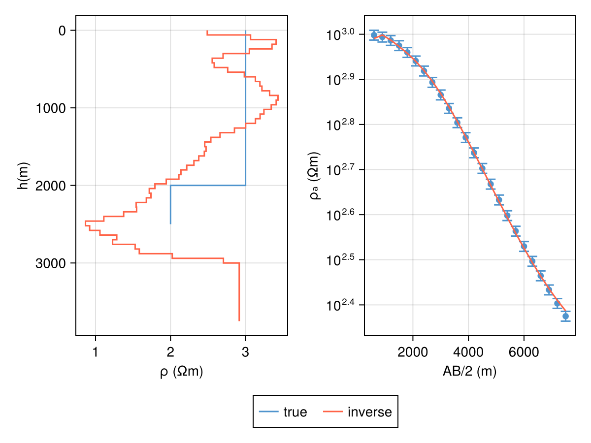
DC Resistivity

We begin by defining a simple synthetic model: with 5 % error floors for Wenner array.

ρ = log10.([1000.0, 100.0])
h = [2000.0]
m = DCModel(ρ, h)

locs = get_wenner_array(400:200:5000)
resp = forward(m, locs)

err_resp = DCResponse(0.05 .* resp.ρₐ)

DCResponse{Vector{Float64}}([49.78080378133154, 49.29938773593118, 48.44937258369504, 47.20042003213615, 45.577483232511035, 43.63801768288286, 41.457587555509846, 39.11689974493678, 36.69228868217137, 34.2502534693876  …  23.26586758159128, 21.46552117101448, 19.81179059476642, 18.301934999175476, 16.93084667959415, 15.691352796166434, 14.57172215520599, 13.560689085508915, 12.654629590939471, 11.854125017539744])

Now, defining an initial model and covariance matrix:

h_test = fill(60.0, 50)
m_lbfgs = DCModel(2.0 .+ zeros(length(h_test) + 1), h_test)

C_d = diagm(inv.(err_resp.ρₐ)) .^ 2

and then

alg_cache = OptAlg(; alg=LBFGS, μ=10.0)
retcode = inverse!(m_lbfgs, resp, locs, alg_cache; W=C_d, max_iters=100);

iteration = 0 : data misfit => 78.24194222644344
iteration = 1 : data misfit => 71.81576783228243
iteration = 2 : data misfit => 56.91681730963348
iteration = 3 : data misfit => 18.90466309892505
iteration = 4 : data misfit => 18.015229709317484
iteration = 5 : data misfit => 14.737884802997224
iteration = 6 : data misfit => 8.738284225812967
iteration = 7 : data misfit => 8.45960731381273
iteration = 8 : data misfit => 8.401195709641975
iteration = 9 : data misfit => 8.35449817789574
iteration = 10 : data misfit => 8.34768954376239
iteration = 11 : data misfit => 8.339653608931851
iteration = 12 : data misfit => 8.332367876563012
iteration = 13 : data misfit => 8.326342566869982
iteration = 14 : data misfit => 8.083499501079396
iteration = 15 : data misfit => 7.767351700531787
iteration = 16 : data misfit => 7.370330614848698
iteration = 17 : data misfit => 7.0690328241306135
iteration = 18 : data misfit => 6.924590538500744
iteration = 19 : data misfit => 6.615917324401324
iteration = 20 : data misfit => 6.314134807558414
iteration = 21 : data misfit => 5.493964626905619
iteration = 22 : data misfit => 3.6417708340063486
iteration = 23 : data misfit => 3.039469890844404
iteration = 24 : data misfit => 2.183401185634076
iteration = 25 : data misfit => 1.9387894325278199
iteration = 26 : data misfit => 2.726224367116941
iteration = 27 : data misfit => 2.5532968282890915
iteration = 28 : data misfit => 2.454263094196572
iteration = 29 : data misfit => 1.7967035923678196
iteration = 30 : data misfit => 1.7061032574214134
iteration = 31 : data misfit => 1.6703720999802996
iteration = 32 : data misfit => 1.5300929276376996
iteration = 33 : data misfit => 1.4235744984887448
iteration = 34 : data misfit => 1.2953302155295279
iteration = 35 : data misfit => 1.1508412505644479
iteration = 36 : data misfit => 0.9124721054644122

Code for this figure

fig = Figure()
ax_m = Axis(fig[1, 1])

plot_model!(ax_m, m; label="true", color=:steelblue3)
plot_model!(ax_m, m_lbfgs; label="inverse", color=:tomato)
fig

ax1 = Axis(fig[1, 2]; xscale=log10)

ab_2 = abs.(locs.srcs[:, 2] .- locs.srcs[:, 1]) ./ 2
plot_response!([ax1], ab_2, resp; plt_type=:scatter, color=:steelblue3)
plot_response!(
    [ax1], ab_2, resp; errs=err_resp, plt_type=:errors, whiskerwidth=10, color=:steelblue3)

resp_lbfgs = forward(m_lbfgs, locs)
plot_response!([ax1], ab_2, resp_lbfgs; color=:tomato)
Legend(fig[2, :], ax_m; orientation=:horizontal)
fig