Variable discretization

There are a few cases when we can simplify the subsurface structure by expressing it using only a few layers. In those cases, it may be desirable to vary the cell size (layer thickness) along with the model parameters. This allows us to move the layer interfaces up and down while parameterizing the model space in a different way wherein there is more flexibility.

Let's denote the model parameters, eg., conductivity, by m, and the layer thickness by h. Therefore, in a N-layer case, we will have

$$\begin{gathered} m=[m_1,m_2,m_3,...,m_N] \\ h=[h_1,h_2,h_3,...,h_{N-1}] \end{gathered}$$

such that

$$\begin{gathered} m_i\in {\mathcal{D}}_{m_i}\text{ ; where }{\mathcal{D}}_{m_i}=\mathit{\text{a priori}}\text{ distribution for }{m}_i\text{ ; and} \\ {h}_i\in {\mathcal{D}}_{h_i}\text{ ; where }{\mathcal{D}}_{h_i}=\mathit{\text{a priori}}\text{ distribution for }{h}_i \end{gathered}$$

In the example that follows, we demonstrate MCMC inversion for a 3-layered earth, including the half-space, imaged using Rayleigh waves. The prior distribution assumes all layers have uncorrelated shear wave velocities bounded between $4.0$ and $5.0km/s$, defined using a uniform distribution, and layer thickness values vary within $\pm 2.5km$ of their nominal values.

!!! tip Important

The most important thing to be noted here is the specification of the prior distribution, done via:

```julia
modelD = RWModelDistribution(
    Product(
        [Uniform(3.5, 5.0) for i in eachindex(z)]
    ),
    Product(
        [Uniform(h_lb[i], h_ub[i]) for i in eachindex(h)]
    )
    ...
);
```

in the example.

Copy-Pasteable code

Let's create a synthetic dataset first, with 1% error floors:

vs = [4.1, 4.4, 4.8]
vp = [7.0, 7.5, 7.8]
ρ = [3.0, 3.2, 3.3]
h = [20.0, 20.0] .* 1e3
m_test = RWModel(vs, h, ρ, vp)

T = exp10.(0:0.1:3)

r_obs = forward(m_test, T);

err_c = 0.01 * r_obs.c;
err_resp = SurfaceWaveResponse(err_c)

Now, let's define the a priori distribution with the variable grid points. Note that we only invert for one physical property, i.e., shear wave velocity.

z = collect(0e3:20e3:40e3)
h = diff(z)
h_ub = h .+ 2.5e3
h_lb = h .- 2.5e3

# variable discretization
modelD = RWModelDistribution(Product([Uniform(4.0, 5.0) for i in eachindex(z)]),
    Product([Uniform(h_lb[i], h_ub[i]) for i in eachindex(h)]),
    fill(3.3, length(z)), fill(7.5, length(z)))

then define the likelihood

respD = SurfaceWaveResponseDistribution(normal_dist)

Put everything together for MCMC

n_samples = 10_000
mcache = mcmc_cache(modelD, respD)

rw_chain = stochastic_inverse(r_obs, err_resp, T, mcache, MH(), n_samples; progress=true)

Chains MCMC chain (10000×8×1 Array{Float64, 3}):

Iterations        = 1:1:10000
Number of chains  = 1
Samples per chain = 10000
Wall duration     = 11.32 seconds
Compute duration  = 11.32 seconds
parameters        = m[:m][1], m[:m][2], m[:m][3], m[:h][1], m[:h][2]
internals         = logprior, loglikelihood, logjoint

Use `describe(chains)` for summary statistics and quantiles.

The obtained rw_chain contains the a posteriori distributions that can be saved using JLD2.jl.

using JLD2
JLD2.@save "file_path.jld2" rw_chain

Code for this figure

fig = Figure()
ax = Axis(fig[1, 1])
hm = get_kde_image!(ax, rw_chain, modelD; kde_transformation_fn=log10,
    grid=(m=collect(4.0:0.01:5.0), z=collect(0:1e3:60e3)),
    trans_utils=(m=no_tf, h=no_tf), colormap=:binary, colorrange=(-4, 0.0))
Colorbar(fig[1, 2], hm; label="log pdf")

mean_kws = (; color=:seagreen3, linewidth=2)
std_kws = (; color=:red, linewidth=1.5)
get_mean_std_image!(
    ax, rw_chain, modelD; confidence_interval=0.9, trans_utils=(m=no_tf, h=no_tf),
    mean_kwargs=mean_kws, std_plus_kwargs=std_kws,
    std_minus_kwargs=std_kws, z_points=collect(0:1e3:60e3))
ylims!(ax, [6e4, 0])

plot_model!(ax, m_test; color=:black, linestyle=:dash, linewidth=2, label="true")
Legend(fig[2, :], ax; orientation=:horizontal)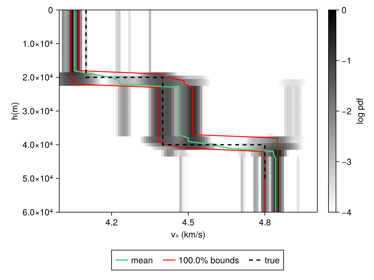

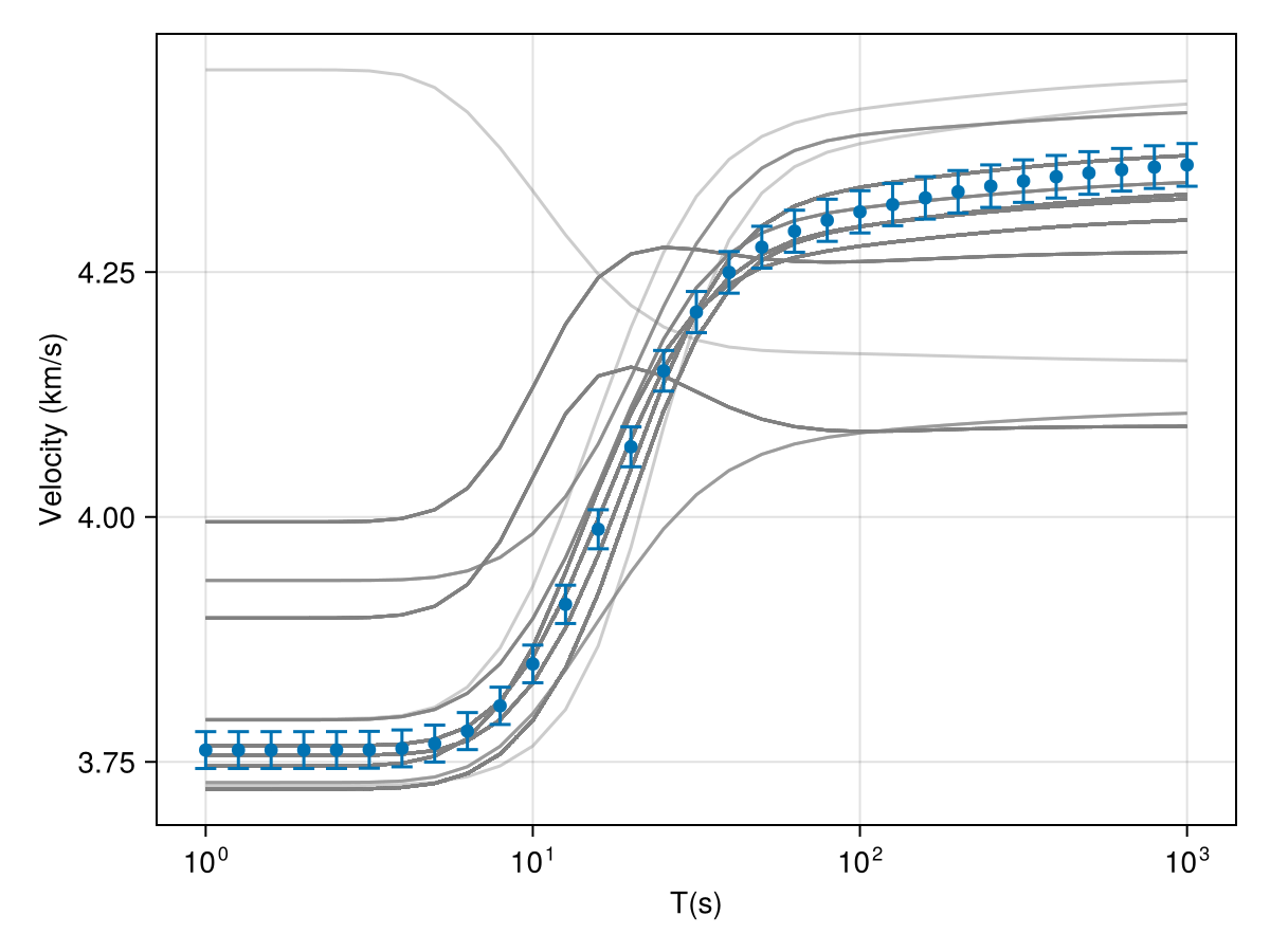
The list of models can then be obtained from chains using, which can then be used to check the fits and perform other diagnostics:

model_list = get_model_list(rw_chain, modelD)

Code for this figure

fig = Figure()
ax1 = Axis(fig[1, 1])

resp_post = forward(model_list[1], T);
for i in 1:(length(model_list) > 1000 ? 1000 : length(model_list))
    forward!(resp_post, model_list[i], T)
    plot_response!([ax1], T, resp_post; alpha=0.4, color=:gray)
end

plot_response!([ax1], T, r_obs; errs=err_resp, plt_type=:errors, whiskerwidth=10)
plot_response!([ax1], T, r_obs; plt_type=:scatter, label="true")