Viscosity models

HK2003

Porosity.HK2003 Type

julia

HK2003(T, P, dg, σ, ϕ, Ch2o_ol = 0.)

Calculate strain rate and viscosity for steady state olivine flow, per Hirth and Kohlstedt (2003), using the three creep mechanisms, i.e., diffusion, dislocation, grain boundary sliding

Arguments

julia

- `T` : Temperature of the rock (K)
- `P` : Pressure (GPa)
- `dg`: Grain size (μm)
- `σ` : Shear stress (GPa)
- `ϕ` : Porosity

Optional Arguments

julia

- `Ch2o_ol` : Water concentration in olivine (ppm), defaults to 0 ppm.

Keyword Arguments

julia

- `params` : Various coefficients required for calculation.
Coefficients for different mechanisms (stored in `mechs` field):
    - `diff` : Diffusion creep
    - `disl` : Dislocation creep
    - `gbs`  : Grain boundary sliding 
To investigate coefficients, call `default_params(Val{HK2003})`. 
To modify coefficients, check the relevant documentation page. This
will also users to get any particular type of mechanism, eg. `diff` only
by setting the `A` in `disl` and `gbs` to `0f0`.

`params` for `HK2003` holds another important field:
- `melt_enhancement` : TODO

Usage

julia

julia> T = collect(1073.0f0:40:1273.0f0);

julia> P = 2 .+ zero(T);

julia> dg = collect(3.0f0:8.0f-1:7.0f0);

julia> σ = collect(7.5f0:1.0f0:12.5f0) .* 1.0f-3;

julia> ϕ = collect(1.0f-2:2.0f-3:2.0f-2);

julia> model = HK2003(T, P, dg, σ, ϕ)
Model : HK2003
Temperature (K) : Float32[1073.0, 1113.0, 1153.0, 1193.0, 1233.0, 1273.0]
Pressure (GPa) : Float32[2.0, 2.0, 2.0, 2.0, 2.0, 2.0]
grain size(μm) : Float32[3.0, 3.8, 4.6, 5.4, 6.2, 7.0]
Shear stress (GPa) : Float32[0.0075000003, 0.0085, 0.009500001, 0.010500001, 0.011500001, 0.0125]
Porosity : Float32[0.01, 0.012, 0.014, 0.016, 0.018, 0.02]
Water concentration in olivine (ppm) : 0.0

julia> forward(model, [])
Rock physics Response : RockphyViscous
Strain rate : Float32[3.152961f-11, 9.076501f-11, 2.643556f-10, 7.560147f-10, 2.093749f-9, 5.5805227f-9]
Viscosity (Pa s) : Float32[2.3787166f17, 9.364843f16, 3.5936449f16, 1.3888621f16, 5.4925405f15, 2.2399335f15]

References

Hirth and Kohlstedt, 2003, "Rheology of the Upper Mantle and the Mantle Wedge: A View from the Experimentalists", Inside the Subduction Factory, J. Eiler (Ed.). https://doi.org/10.1029/138GM06

source

Varying grain size

The distribution with temperature looks like (assuming increase in grain size is independent of other parameters) at 2 GPa pressure with a porosity of 0.015:

Code for this figure

julia

f = Figure(; size=(700, 400))

T = (600:1600) .+ 273.0
P = 2.0
dg = [1.0, 3.0, 10.0, 30.0]'
σ = 10e-3
ϕ = 0.015

m = HK2003(T, P, dg, σ, ϕ)
resp = forward(m, []);

resp_fields = [:ϵ_rate, :η]
units = ["", "(Pa s)"]

ax_coords = [(1, 1), (1, 2)]
for i in eachindex(resp_fields)
    ax = Axis(f[ax_coords[i]...]; xlabel="10⁴/T (K⁻¹)",
        ylabel=string(resp_fields[i]) * " $(units[i])",
        yticks=LogTicks(WilkinsonTicks(6; k_min=5)), backgroundcolor=(:magenta, 0.052))

    xts = inv.([600, 800, 1000, 1200, 1600] .+ 273.0) .* 1e4

    ax2 = Axis(
        f[ax_coords[i]...]; xaxisposition=:top, yaxisposition=:right, xlabel="T (ᴼC)",
        xgridvisible=false, xtickformat=x -> string.(round.((1e4 ./ x) .- 273)),
        xticklabelsize=8, backgroundcolor=(:magenta, 0.05))
    ax2.xticks = xts
    hidespines!(ax2)
    hideydecorations!(ax2)
    linkyaxes!(ax, ax2)
    ylims!(ax, extrema(getfield(resp, resp_fields[i])) .* (0.3, 3))
    ylims!(ax2, extrema(getfield(resp, resp_fields[i])) .* (0.3, 3))
    ax.yscale = log10
    ax2.yscale = log10

    for j in axes(getfield(resp, resp_fields[i]), 2)
        d = dg[j]
        r_ = getfield(resp, resp_fields[i])
        lines!(ax, inv.(T) .* 1e4, r_[:, j]; label="$d")
        lines!(ax2, inv.(T) .* 1e4, r_[:, j]; alpha=0)
    end
end
f[2, 1:2] = Legend(f, f.content[end - 1], "grain size (μm)"; orientation=:horizontal)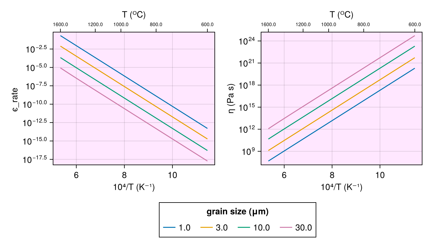

Varying porosity

We can also look at the distribution with parameters by varying just the porosity :

Code for this figure

julia

f = Figure(; size=(700, 400))

T = (600:1600) .+ 273.0
P = 2.0
dg = 4.0
σ = 10e-3
ϕ = [0.01, 0.03, 0.1, 0.3]'

m = HK2003(T, P, dg, σ, ϕ)
resp = forward(m, []);

resp_fields = [:ϵ_rate, :η]
units = ["", "(Pa⋅s)"]

ax_coords = [(1, 1), (1, 2)]
for i in eachindex(resp_fields)
    ax = Axis(f[ax_coords[i]...]; xlabel="10⁴/T (K⁻¹)",
        ylabel=string(resp_fields[i]) * " $(units[i])",
        yticks=LogTicks(WilkinsonTicks(6; k_min=5)), backgroundcolor=(:magenta, 0.052))

    xts = inv.([600, 800, 1000, 1200, 1600] .+ 273.0) .* 1e4

    ax2 = Axis(
        f[ax_coords[i]...]; xaxisposition=:top, yaxisposition=:right, xlabel="T (ᴼC)",
        xgridvisible=false, xtickformat=x -> string.(round.((1e4 ./ x) .- 273)),
        xticklabelsize=8, backgroundcolor=(:magenta, 0.05))
    ax2.xticks = xts
    hidespines!(ax2)
    hideydecorations!(ax2)
    linkyaxes!(ax, ax2)
    ylims!(ax, extrema(getfield(resp, resp_fields[i])) .* (0.3, 3))
    ylims!(ax2, extrema(getfield(resp, resp_fields[i])) .* (0.3, 3))
    ax.yscale = log10
    ax2.yscale = log10

    for j in axes(getfield(resp, resp_fields[i]), 2)
        d = ϕ[j]
        r_ = getfield(resp, resp_fields[i])
        lines!(ax, inv.(T) .* 1e4, r_[:, j]; label="$d")
        lines!(ax2, inv.(T) .* 1e4, r_[:, j]; alpha=0)
    end
end
f[2, 1:2] = Legend(f, f.content[end - 1], "porosity"; orientation=:horizontal)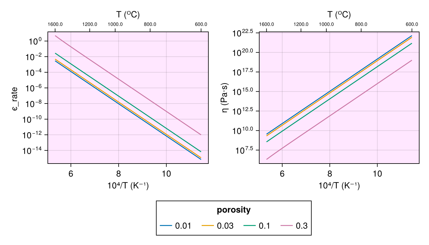

Varying water content

Another important parameter to consider for HK2003 is water content. By default, we assume 0 ppm. The distribution with temperature for different water content (keeping other parameters constant) looks like :

Code for this figure

julia

f = Figure(; size=(700, 400))

T = (600:1600) .+ 273.0
P = 2.0
dg = 4.0
σ = 10e-3
ϕ = 0.015
Ch2o = [0.0, 100.0, 300.0, 1000.0]'

m = HK2003(T, P, dg, σ, ϕ, Ch2o)
resp = forward(m, []);

resp_fields = [:ϵ_rate, :η]
units = ["", "(Pa⋅s)"]

ax_coords = [(1, 1), (1, 2)]
for i in eachindex(resp_fields)
    ax = Axis(f[ax_coords[i]...]; xlabel="10⁴/T (K⁻¹)",
        ylabel=string(resp_fields[i]) * " $(units[i])",
        yticks=LogTicks(WilkinsonTicks(6; k_min=5)), backgroundcolor=(:magenta, 0.052))

    xts = inv.([600, 800, 1000, 1200, 1600] .+ 273.0) .* 1e4

    ax2 = Axis(
        f[ax_coords[i]...]; xaxisposition=:top, yaxisposition=:right, xlabel="T (ᴼC)",
        xgridvisible=false, xtickformat=x -> string.(round.((1e4 ./ x) .- 273)),
        xticklabelsize=8, backgroundcolor=(:magenta, 0.05))
    ax2.xticks = xts
    hidespines!(ax2)
    hideydecorations!(ax2)
    linkyaxes!(ax, ax2)
    ylims!(ax, extrema(getfield(resp, resp_fields[i])) .* (0.3, 3))
    ylims!(ax2, extrema(getfield(resp, resp_fields[i])) .* (0.3, 3))
    ax.yscale = log10
    ax2.yscale = log10

    for j in axes(getfield(resp, resp_fields[i]), 2)
        d = Ch2o[j]
        r_ = getfield(resp, resp_fields[i])
        lines!(ax, inv.(T) .* 1e4, r_[:, j]; label="$d")
        lines!(ax2, inv.(T) .* 1e4, r_[:, j]; alpha=0)
    end
end
f[2, 1:2] = Legend(f, f.content[end - 1], "Water conc. (ppm)"; orientation=:horizontal)

HZK2011

Porosity.HZK2011 Type

julia

HZK2011(T, P, dg, σ, ϕ)

Calculate strain rate and viscosity for steady state olivine flow, per Zimmerman and Kohlstedt (2011), using the three creep mechanisms, i.e., diffusion, dislocation, grain boundary sliding

Arguments

julia

- `T` : Temperature of the rock (K)
- `P` : Pressure (GPa)
- `dg`: Grain size (μm)
- `σ` : Shear stress (GPa)
- `ϕ` : Porosity

Keyword Arguments

julia

- `params` : Various coefficients required for calculation.
Coefficients for different mechanisms (stored in `mechs` field):
    - `diff` : Diffusion creep
    - `disl` : Dislocation creep
    - `gbs`  : Grain boundary sliding 
To investigate coefficients, call `default_params(Val{HZK2011})`. 
To modify coefficients, check the relevant documentation page. This
will also users to get any particular type of mechanism, eg. `diff` only
by setting the `A` in `disl` and `gbs` to `0f0`.

`params` for `HZK2011` holds another important field:
    - `melt_enhancement` : TODO

Usage

julia

julia> T = collect(1073.0f0:40:1273.0f0);

julia> P = 2 .+ zero(T);

julia> dg = collect(3.0f0:8.0f-1:7.0f0);

julia> σ = collect(7.5f0:1.0f0:12.5f0) .* 1.0f-3;

julia> ϕ = collect(1.0f-2:2.0f-3:2.0f-2);

julia> model = HZK2011(T, P, dg, σ, ϕ)
Model : HZK2011
Temperature (K) : Float32[1073.0, 1113.0, 1153.0, 1193.0, 1233.0, 1273.0]
Pressure (GPa) : Float32[2.0, 2.0, 2.0, 2.0, 2.0, 2.0]
grain size(μm) : Float32[3.0, 3.8, 4.6, 5.4, 6.2, 7.0]
Shear stress (GPa) : Float32[0.0075000003, 0.0085, 0.009500001, 0.010500001, 0.011500001, 0.0125]
Porosity : Float32[0.01, 0.012, 0.014, 0.016, 0.018, 0.02]

julia> forward(model, [])
Rock physics Response : RockphyViscous
Strain rate : Float32[8.3687815f-13, 2.4096476f-12, 7.02197f-12, 2.0106366f-11, 5.5824817f-11, 1.4951564f-10]
Viscosity (Pa s) : Float32[8.961879f18, 3.5274867f18, 1.3528968f18, 5.222227f17, 2.060016f17, 8.36033f16]

References

Hansen, Zimmerman and Kohlstedt, 2011, "Grain boundary sliding in San Carlos olivine: Flow law parameters and crystallographic-preferred orientation", J. Geophys. Res., https://doi.org/10.1029/2011JB008220

source

Varying grain size

The distribution with temperature looks like (assuming increase in grain size is independent of other parameters) at 2 GPa pressure with a porosity of 0.015:

Code for this figure

julia

f = Figure(; size=(700, 400))

T = (600:1600) .+ 273.0
P = 2.0
dg = [1.0, 3.0, 10.0, 30.0]'
σ = 10e-3
ϕ = 0.015

m = HZK2011(T, P, dg, σ, ϕ)
resp = forward(m, []);

resp_fields = [:ϵ_rate, :η]
units = ["", "(Pa s)"]

ax_coords = [(1, 1), (1, 2)]
for i in eachindex(resp_fields)
    ax = Axis(f[ax_coords[i]...]; xlabel="10⁴/T (K⁻¹)",
        ylabel=string(resp_fields[i]) * " $(units[i])",
        yticks=LogTicks(WilkinsonTicks(6; k_min=5)), backgroundcolor=(:magenta, 0.052))

    xts = inv.([600, 800, 1000, 1200, 1600] .+ 273.0) .* 1e4

    ax2 = Axis(
        f[ax_coords[i]...]; xaxisposition=:top, yaxisposition=:right, xlabel="T (ᴼC)",
        xgridvisible=false, xtickformat=x -> string.(round.((1e4 ./ x) .- 273)),
        xticklabelsize=8, backgroundcolor=(:magenta, 0.05))
    ax2.xticks = xts
    hidespines!(ax2)
    hideydecorations!(ax2)
    linkyaxes!(ax, ax2)
    ylims!(ax, extrema(getfield(resp, resp_fields[i])) .* (0.3, 3))
    ylims!(ax2, extrema(getfield(resp, resp_fields[i])) .* (0.3, 3))
    ax.yscale = log10
    ax2.yscale = log10

    for j in axes(getfield(resp, resp_fields[i]), 2)
        d = dg[j]
        r_ = getfield(resp, resp_fields[i])
        lines!(ax, inv.(T) .* 1e4, r_[:, j]; label="$d")
        lines!(ax2, inv.(T) .* 1e4, r_[:, j]; alpha=0)
    end
end
f[2, 1:2] = Legend(f, f.content[end - 1], "grain size (μm)"; orientation=:horizontal)

Varying porosity

We can also look at the distribution with parameters by varying just the porosity :

Code for this figure

julia

f = Figure(; size=(700, 400))

T = (600:1600) .+ 273.0
P = 2.0
dg = 4.0
σ = 10e-3
ϕ = [0.01, 0.03, 0.1, 0.3]'

m = HZK2011(T, P, dg, σ, ϕ)
resp = forward(m, []);

resp_fields = [:ϵ_rate, :η]
units = ["", "(Pa⋅s)"]

ax_coords = [(1, 1), (1, 2)]
for i in eachindex(resp_fields)
    ax = Axis(f[ax_coords[i]...]; xlabel="10⁴/T (K⁻¹)",
        ylabel=string(resp_fields[i]) * " $(units[i])",
        yticks=LogTicks(WilkinsonTicks(6; k_min=5)), backgroundcolor=(:magenta, 0.052))

    xts = inv.([600, 800, 1000, 1200, 1600] .+ 273.0) .* 1e4

    ax2 = Axis(
        f[ax_coords[i]...]; xaxisposition=:top, yaxisposition=:right, xlabel="T (ᴼC)",
        xgridvisible=false, xtickformat=x -> string.(round.((1e4 ./ x) .- 273)),
        xticklabelsize=8, backgroundcolor=(:magenta, 0.05))
    ax2.xticks = xts
    hidespines!(ax2)
    hideydecorations!(ax2)
    linkyaxes!(ax, ax2)
    ylims!(ax, extrema(getfield(resp, resp_fields[i])) .* (0.3, 3))
    ylims!(ax2, extrema(getfield(resp, resp_fields[i])) .* (0.3, 3))
    ax.yscale = log10
    ax2.yscale = log10

    for j in axes(getfield(resp, resp_fields[i]), 2)
        d = ϕ[j]
        r_ = getfield(resp, resp_fields[i])
        lines!(ax, inv.(T) .* 1e4, r_[:, j]; label="$d")
        lines!(ax2, inv.(T) .* 1e4, r_[:, j]; alpha=0)
    end
end
f[2, 1:2] = Legend(f, f.content[end - 1], "porosity"; orientation=:horizontal)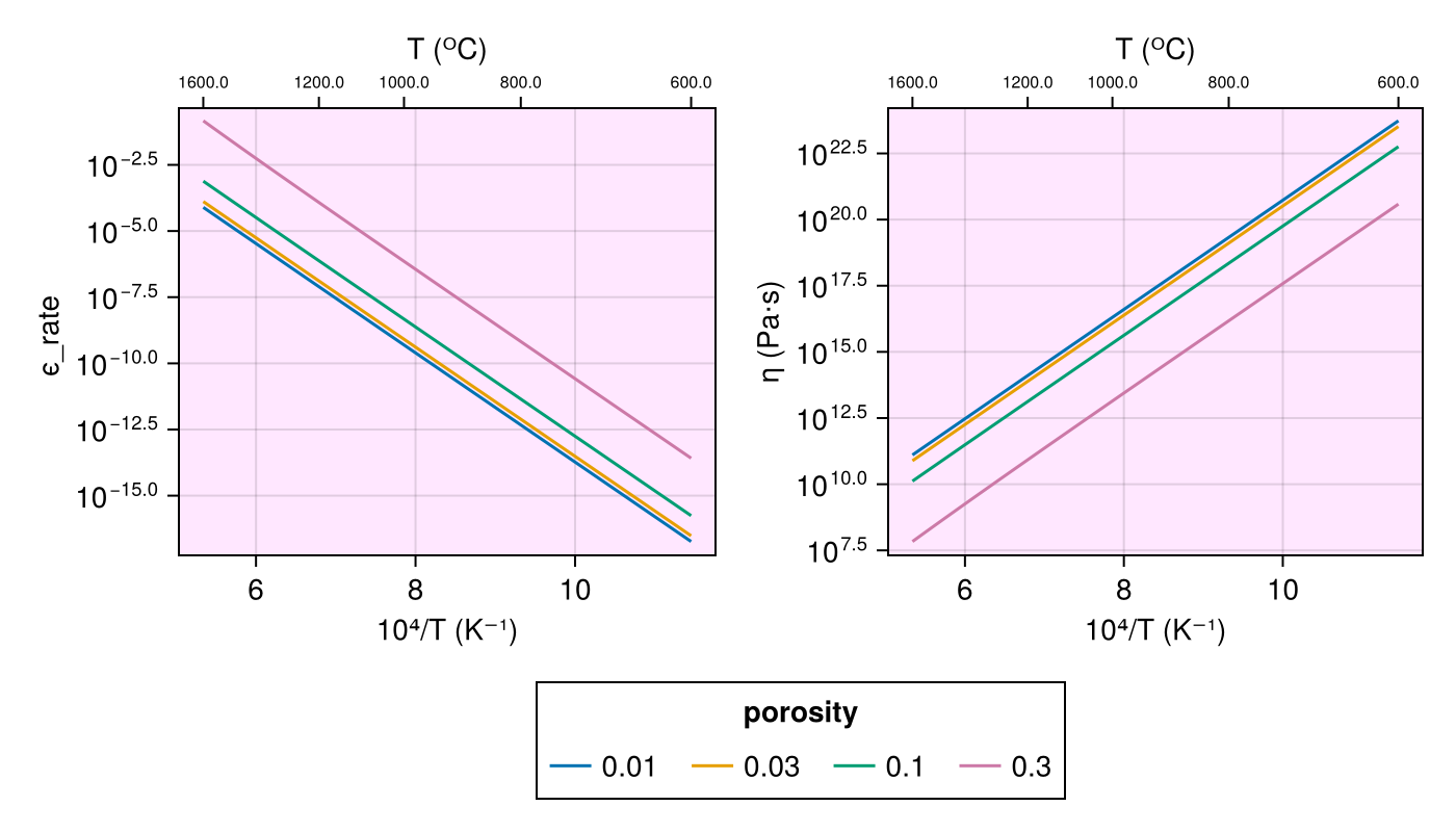

xfit_premelt

Porosity.xfit_premelt Type

julia

xfit_premelt(T, P, dg, σ, ϕ)

Calculate viscosity for steady state olivine flow for pre-melting, i.e., temperatures are just below and above the solidus, per Yamauchi and Takei (2016)

Arguments

julia

- `T` : Temperature of the rock (K)
- `P` : Pressure (GPa)
- `dg`: Grain size (μm)
- `σ` : Shear stress (GPa)
- `ϕ` : Porosity
- `T_solidus` : Solidus temperature

Keyword Arguments

julia

- `params` : Various coefficients required for calculation.
Coefficients for different mechanisms (stored in `mechs` field):
    - `diff` : Diffusion creep
    - `disl` : Dislocation creep
    - `gbs`  : Grain boundary sliding 
To investigate coefficients, call `default_params(Val{xfit_premelt}())`. 
To modify coefficients, check the relevant documentation page. This
will also users to get any particular type of mechanism, eg. `diff` only
by setting the `A` in `disl` and `gbs` to `0f0`.

Usage

julia

julia> T = collect(1073.0f0:40:1273.0f0);

julia> P = 2 .+ zero(T);

julia> dg = collect(3.0f0:8.0f-1:7.0f0);

julia> σ = collect(7.5f0:1.0f0:12.5f0) .* 1.0f-3;

julia> ϕ = collect(1.0f-2:2.0f-3:2.0f-2);

julia> T_solidus = 1200 + 273 .+ zero(T);

julia> model = xfit_premelt(T, P, dg, σ, ϕ, T_solidus)
Model : xfit_premelt
Temperature (K) : Float32[1073.0, 1113.0, 1153.0, 1193.0, 1233.0, 1273.0]
Pressure (GPa) : Float32[2.0, 2.0, 2.0, 2.0, 2.0, 2.0]
grain size(μm) : Float32[3.0, 3.8, 4.6, 5.4, 6.2, 7.0]
Shear stress (GPa) : Float32[0.0075000003, 0.0085, 0.009500001, 0.010500001, 0.011500001, 0.0125]
Porosity : Float32[0.01, 0.012, 0.014, 0.016, 0.018, 0.02]
Solidus Temperature (K) : Float32[1473.0, 1473.0, 1473.0, 1473.0, 1473.0, 1473.0]

julia> forward(model, [])
Rock physics Response : RockphyViscous
Strain rate : Float32[0.0, 0.0, 0.0, 0.0, 0.0, 0.0]
Viscosity (Pa s) : Float32[7.6341115f18, 2.2587335f18, 6.6676584f17, 2.024383f17, 6.40973f16, 2.1291828f16]

References

Yamauchi and Takei, 2016, "Polycrystal anelasticity at near-solidus temperatures", J. Geophys. Res. Solid Earth, https://doi.org/10.1002/2016JB013316

source

!!!note

Note that `xfit_premelt` populates the return value of strain rate with zeros. We, therefore, do not plot the same here.

Varying grain size

The distribution with temperature looks like (assuming increase in grain size is independent of other parameters) at 2 GPa pressure with a porosity of 0.015 at solidus temperature of 1200 ᴼC:

Code for this figure

julia

f = Figure(; size=(600, 400))

T = (600:1600) .+ 273.0
P = 2.0
dg = [1.0, 3.0, 10.0, 30.0]'
σ = 10e-3
ϕ = 0.015
T_solidus = 1200 + 273

m = xfit_premelt(T, P, dg, σ, ϕ, T_solidus)
resp = forward(m, []);

resp_fields = [:η]
units = ["(Pa s)"]

ax_coords = [(1, 1), (1, 2)]
for i in eachindex(resp_fields)
    ax = Axis(f[ax_coords[i]...]; xlabel="10⁴/T (K⁻¹)",
        ylabel=string(resp_fields[i]) * " $(units[i])",
        yticks=LogTicks(WilkinsonTicks(6; k_min=5)), backgroundcolor=(:magenta, 0.052))

    xts = inv.([600, 800, 1000, 1200, 1600] .+ 273.0) .* 1e4

    ax2 = Axis(
        f[ax_coords[i]...]; xaxisposition=:top, yaxisposition=:right, xlabel="T (ᴼC)",
        xgridvisible=false, xtickformat=x -> string.(round.((1e4 ./ x) .- 273)),
        xticklabelsize=8, backgroundcolor=(:magenta, 0.05))
    ax2.xticks = xts
    hidespines!(ax2)
    hideydecorations!(ax2)
    linkyaxes!(ax, ax2)

    if sum(extrema(getfield(resp, resp_fields[i]))) > 1e-15
        ylims!(ax, extrema(getfield(resp, resp_fields[i])) .* (0.3, 3))
        ylims!(ax2, extrema(getfield(resp, resp_fields[i])) .* (0.3, 3))
        ax.yscale = log10
        ax2.yscale = log10
    end
    for j in axes(getfield(resp, resp_fields[i]), 2)
        d = dg[j]
        r_ = getfield(resp, resp_fields[i])
        lines!(ax, inv.(T) .* 1e4, r_[:, j]; label="$d")
        lines!(ax2, inv.(T) .* 1e4, r_[:, j]; alpha=0)
    end
end

f[1, 2] = Legend(f, f.content[end - 1], "grain size (μm)")

for i in eachindex(f.content[1:(end - 1)])
    ax_ = f.content[i]
    lv = vlines!(ax_, 1e4 / T_solidus; color=:green, linestyle=:dash)
    axislegend(
        ax_, [lv], ["solidus temperature"]; position=:rb, labelsize=12, framevisible=false)
end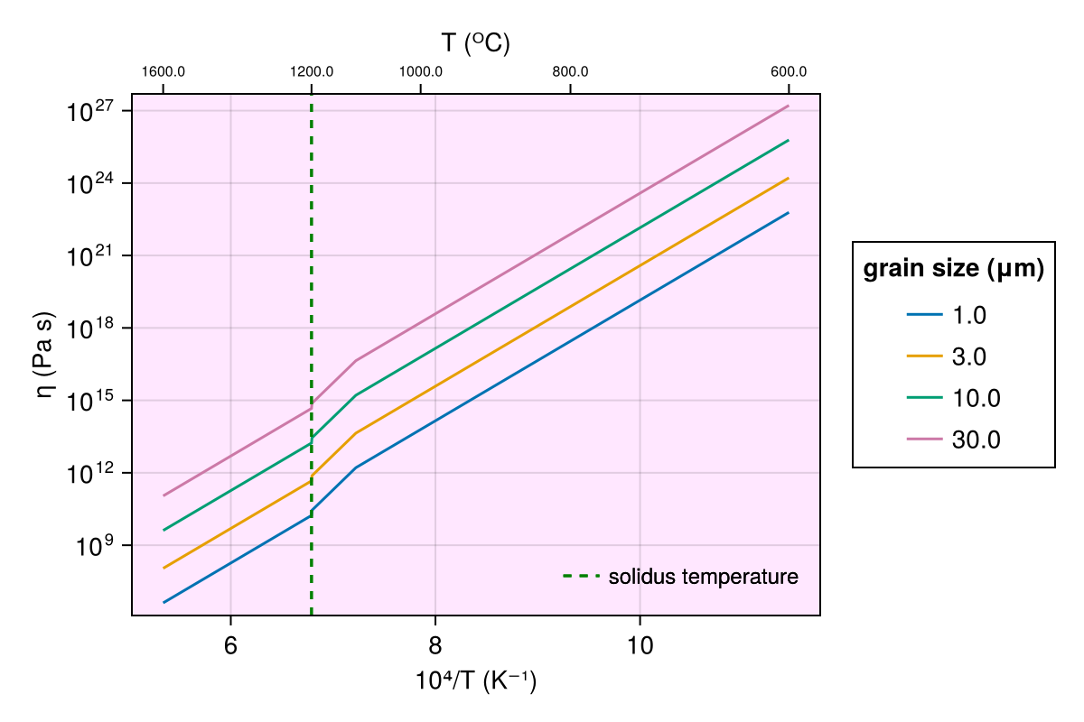

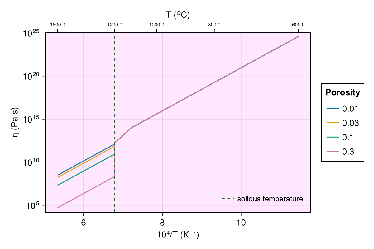
Varying porosity

We can also look at the distribution with parameters by varying just the porosity :

Code for this figure

julia

f = Figure(; size=(600, 400))

T = (600:1600) .+ 273.0
P = 2.0
dg = 4.0
σ = 10e-3
ϕ = [0.01, 0.03, 0.1, 0.3]'
T_solidus = 1200 + 273

m = xfit_premelt(T, P, dg, σ, ϕ, T_solidus)
resp = forward(m, []);

resp_fields = [:η]
units = ["(Pa s)"]

ax_coords = [(1, 1), (1, 2)]
for i in eachindex(resp_fields)
    ax = Axis(f[ax_coords[i]...]; xlabel="10⁴/T (K⁻¹)",
        ylabel=string(resp_fields[i]) * " $(units[i])",
        yticks=LogTicks(WilkinsonTicks(6; k_min=5)), backgroundcolor=(:magenta, 0.052))

    xts = inv.([600, 800, 1000, 1200, 1600] .+ 273.0) .* 1e4

    ax2 = Axis(
        f[ax_coords[i]...]; xaxisposition=:top, yaxisposition=:right, xlabel="T (ᴼC)",
        xgridvisible=false, xtickformat=x -> string.(round.((1e4 ./ x) .- 273)),
        xticklabelsize=8, backgroundcolor=(:magenta, 0.05))
    ax2.xticks = xts
    hidespines!(ax2)
    hideydecorations!(ax2)
    linkyaxes!(ax, ax2)

    if sum(extrema(getfield(resp, resp_fields[i]))) > 1e-15
        ylims!(ax, extrema(getfield(resp, resp_fields[i])) .* (0.3, 3))
        ylims!(ax2, extrema(getfield(resp, resp_fields[i])) .* (0.3, 3))
        ax.yscale = log10
        ax2.yscale = log10
    end
    for j in axes(getfield(resp, resp_fields[i]), 2)
        d = ϕ[j]
        r_ = getfield(resp, resp_fields[i])
        lines!(ax, inv.(T) .* 1e4, r_[:, j]; label="$d")
        lines!(ax2, inv.(T) .* 1e4, r_[:, j]; alpha=0)
    end
end

f[1, 2] = Legend(f, f.content[end - 1], "Porosity")

for i in eachindex(f.content[1:(end - 1)])
    ax_ = f.content[i]
    lv = vlines!(ax_, 1e4 / T_solidus; color=:green, linestyle=:dash)
    axislegend(
        ax_, [lv], ["solidus temperature"]; position=:rb, labelsize=12, framevisible=false)
end

Viscosity models ​

HK2003 ​

Varying grain size ​

Varying porosity ​

Varying water content ​

HZK2011 ​

Varying grain size ​

Varying porosity ​

xfit_premelt ​

Varying grain size ​

Varying porosity ​

Viscosity models

HK2003

Varying grain size

Varying porosity

Varying water content

HZK2011

Varying grain size

Varying porosity

xfit_premelt

Varying grain size

Varying porosity