Combine models
We provide the feature to model multiple rock physics simultaneously. This is useful because often we want to model, say electrical conductivity and p-wave velocity, for the same temperatures, melt fraction, water content and other parameters. This utility showcases itself particularly when we want to perform the stochastic inversion of rock physics properties. For now, lets understand how to get the responses from multi rock physics models.
Please note that this bears close resemblance with Mixing phases tutorial. :::
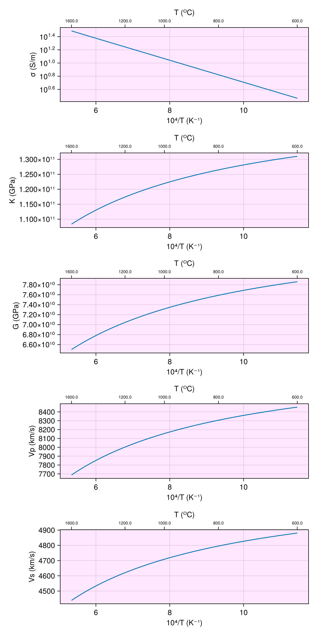
We first need to define the rock physics we want to model. To model electrical conductivity using SEO3 and elastic properties using anharmonic, we use multi_rp_modelType
m = multi_rp_modelType(SEO3, anharmonic, Nothing, Nothing)multi_rp_modelType{SEO3, anharmonic, Nothing, Nothing}(SEO3, anharmonic, Nothing, Nothing)The multi_rp_modelType function requires exactly 4 parameters, first of which defines the conductivity model, followed by elastic, viscous and anelastic models in that order. To exclude the physics of any kind, pass Nothing in its place, e.g., in the above example, we have SEO3 for conductivity and anharmonic for elastic. Since we did not want to model viscous and anelastic responses, we passed Nothing in their places.
Now, we define the parameters required to define the model.
T = (600:1600) .+ 273.0f0
P = 3.0f0
ρ = 3300.0f0
ϕ = 0.1f0

ps_nt = (; T=T, P=P, ρ=ρ, ϕ=ϕ)
model = m(ps_nt)
and then as usual get the response
resp = forward(model, [])Code for this figure
f = Figure(; size=(600, 1200))

resp_nt = Porosity.to_resp_nt(resp)

resp_fields = [:σ, :K, :G, :Vp, :Vs]
units = ["S/m", "GPa", "GPa", "km/s", "km/s"]

ax_coords = [(1, 1), (2, 1), (3, 1), (4, 1), (5, 1)]
for i in eachindex(resp_fields)
    ax = Axis(f[ax_coords[i]...]; xlabel="10⁴/T (K⁻¹)",
        ylabel=string(resp_fields[i]) * " ($(units[i]))",
        yticks=LogTicks(WilkinsonTicks(6; k_min=5)), backgroundcolor=(:magenta, 0.052))

    xts = inv.([600, 800, 1000, 1200, 1600] .+ 273.0) .* 1e4

    ax2 = Axis(
        f[ax_coords[i]...]; xaxisposition=:top, yaxisposition=:right, xlabel="T (ᴼC)",
        xgridvisible=false, xtickformat=x -> string.(round.((1e4 ./ x) .- 273)),
        xticklabelsize=8, backgroundcolor=(:magenta, 0.05))
    ax2.xticks = xts
    hidespines!(ax2)
    hideydecorations!(ax2)
    linkyaxes!(ax, ax2)

    r_ = getfield(resp_nt, resp_fields[i])
    if i == 1
        lines!(ax, inv.(T) .* 1e4, 10.0 .^ r_)
        lines!(ax2, inv.(T) .* 1e4, 10.0 .^ r_; alpha=0)
        ax.yscale = log10
        ax2.yscale = log10
    else
        lines!(ax, inv.(T) .* 1e4, r_)
        lines!(ax2, inv.(T) .* 1e4, r_; alpha=0)
    end
end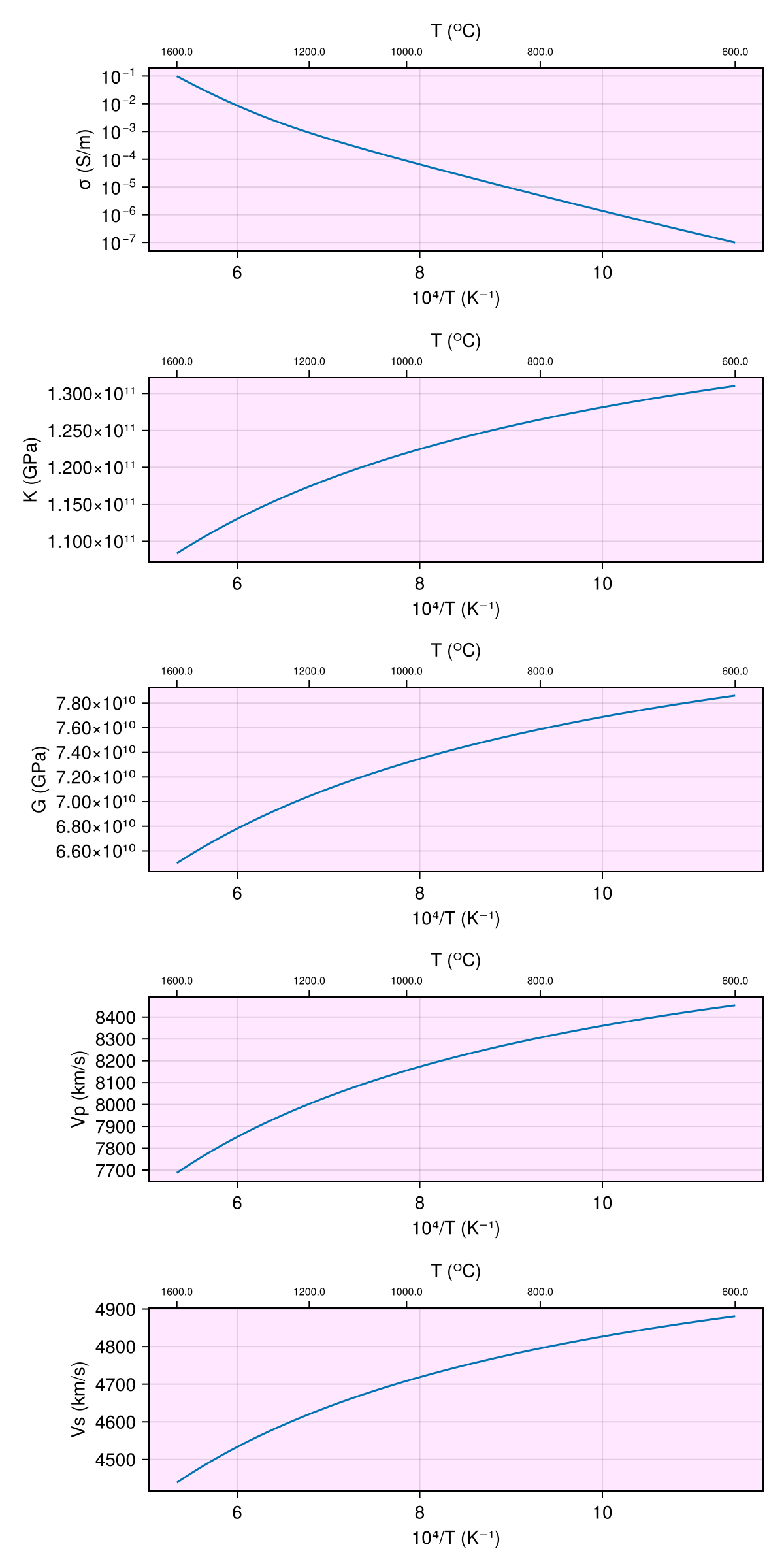
Bonus example !!
Sooner or later, you would want to also mix phases in estimating conductivity. The logic for constructing the model type and the model is also same. We first need to define the mixing type
m_mix = two_phase_modelType(SEO3, Gaillard2008, HS1962_plus)two_phase_modelType{SEO3, Gaillard2008, HS1962_plus}(SEO3, Gaillard2008, HS1962_plus)and then construct the multi rock physics type
m = multi_rp_modelType(typeof(m_mix), anharmonic, Nothing, Nothing)multi_rp_modelType{two_phase_modelType{SEO3, Gaillard2008, HS1962_plus}, anharmonic, Nothing, Nothing}(two_phase_modelType{SEO3, Gaillard2008, HS1962_plus}, anharmonic, Nothing, Nothing)and then throw in the parameters
T = (600:1600) .+ 273.0f0
P = 3.0f0
ρ = 3300.0f0
ϕ = 0.1f0

ps_nt = (; T=T, P=P, ρ=ρ, ϕ=ϕ)
model = m(ps_nt)
and then as usual get the response
resp = forward(model, [])Code for this figure
f = Figure(; size=(600, 1200))

resp_nt = Porosity.to_resp_nt(resp)

resp_fields = [:σ, :K, :G, :Vp, :Vs]
units = ["S/m", "GPa", "GPa", "km/s", "km/s"]

ax_coords = [(1, 1), (2, 1), (3, 1), (4, 1), (5, 1)]
for i in eachindex(resp_fields)
    ax = Axis(f[ax_coords[i]...]; xlabel="10⁴/T (K⁻¹)",
        ylabel=string(resp_fields[i]) * " ($(units[i]))",
        yticks=LogTicks(WilkinsonTicks(6; k_min=5)), backgroundcolor=(:magenta, 0.052))

    xts = inv.([600, 800, 1000, 1200, 1600] .+ 273.0) .* 1e4

    ax2 = Axis(
        f[ax_coords[i]...]; xaxisposition=:top, yaxisposition=:right, xlabel="T (ᴼC)",
        xgridvisible=false, xtickformat=x -> string.(round.((1e4 ./ x) .- 273)),
        xticklabelsize=8, backgroundcolor=(:magenta, 0.05))
    ax2.xticks = xts
    hidespines!(ax2)
    hideydecorations!(ax2)
    linkyaxes!(ax, ax2)

    r_ = getfield(resp_nt, resp_fields[i])
    if i == 1
        lines!(ax, inv.(T) .* 1e4, 10.0 .^ r_)
        lines!(ax2, inv.(T) .* 1e4, 10.0 .^ r_; alpha=0)
        ax.yscale = log10
        ax2.yscale = log10
    else
        lines!(ax, inv.(T) .* 1e4, r_)
        lines!(ax2, inv.(T) .* 1e4, r_; alpha=0)
    end
end