Tuning rock physics hyperparameters

A dependency scenario

When the temperatures get high enough and near the solidus temperature to start melting, the melt fraction no longer remains an independent variable. Similarly, addition of volatiles implies solidus temperature itself is a function of volatile concentration. This in turn, implies melt fraction is a function of volatile concentration along with the temperature.

Depending on the type of model chosen for estimating solidus temperature, then consequently melt fraction and the partition coefficients as well, the estimates of melt fraction changes and so do these parameters as well. This makes it challenging to model such functions. In order to tune the rock physics parameters where one of the variables are dependent on another, we provide tune_rp_modelType

Porosity.tune_rp_modelType Type

tune_rp_modelType(fn_list, mtype)

Arguments

• fn_list : Vector of functions applied to the parameters in the same sequence

• mtype : model type that will constructed using the given and estimated parameters

Usage

julia> T = (800:200:1200) .+ 273.0;

julia> P = 2.0;

julia> T_solidus = 1000.0 + 273;

julia> ps_nt = (; T=T, P=P, T_solidus=T_solidus);

julia> fn_list = [get_melt_fraction];

julia> m_type = two_phase_modelType(SEO3, Gaillard2008, HS1962_plus);

julia> m = tune_rp_modelType(fn_list, m_type)
Tuning rock physics with function list :
[Porosity.get_melt_fraction]
to obtain the rock physics model of type two_phase_modelType{SEO3, Gaillard2008, HS1962_plus}

julia> model = m(ps_nt)
Two phase composition using HS1962_plus()

*    m₁ (solid phase) : 
Model : SEO3
Temperature (K) : 1073.0:200.0:1473.0
ϕ : [1.0, 1.0, 0.4594594594594593]

*    m₂ (liquid phase) : 
Model : SEO3
Temperature (K) : 1073.0:200.0:1473.0
ϕ : [0.0, 0.0, 0.5405405405405407]

source

Example

tune_rp_model has a vector/list of functions as the first argument. These functions are applied in the order of their positions in the list to the input arguments are made available to the model, the second argument of tune_rp_model. The variables for input are given through a named tuple.

The following example demonstrates the utility. Let's first define the parameters :

T = (800:1200) .+ 273.0
P = 2.0
T_solidus = 1000.0 + 273

ps_nt = (; T=T, P=P, T_solidus=T_solidus)

(T = 1073.0:1.0:1473.0, P = 2.0, T_solidus = 1273.0)

We calculate the melt fraction using get_melt_fraction, and then using the estimated melt fraction, calculate the bulk conductivity using Hashin-Shtrikman upper bound.

fn_list = [get_melt_fraction]
m_type = two_phase_modelType(SEO3, Gaillard2008, HS1962_plus)
m = tune_rp_modelType(fn_list, m_type)

model = m(ps_nt)

Calculating the forward response is then done as usual :

resp = forward(model, [])

Code for this figure

f = Figure()
ax = Axis(f[1, 1]; yscale=log10, xlabel="10⁴/T (K⁻¹)", ylabel="σ (S/m)",
    yticks=LogTicks(WilkinsonTicks(9; k_min=8)), backgroundcolor=(:magenta, 0.05))

xts = inv.([300, 600, 900, 1200, 1500] .+ 273.0) .* 1e4

ax2 = Axis(f[1, 1]; yscale=log10, xaxisposition=:top, yaxisposition=:right, xlabel="T (ᴼC)",
    xgridvisible=false, xtickformat=x -> string.(round.((1e4 ./ x) .- 273)),
    xticklabelsize=10, backgroundcolor=(:magenta, 0.05))
ax2.xticks = xts
hidespines!(ax2)
hideydecorations!(ax2)
linkyaxes!(ax, ax2)

logsig = resp.σ

lines!(ax, inv.(T) .* 1e4, 10 .^ logsig)
lines!(ax2, inv.(T) .* 1e4, 10 .^ logsig; alpha=0)

ylims!(ax, 1e-8, 1)
ylims!(ax2, 1e-8, 1e4)

┌ Warning: No strict ticks found
└ @ PlotUtils ~/.julia/packages/PlotUtils/HX80C/src/ticks.jl:194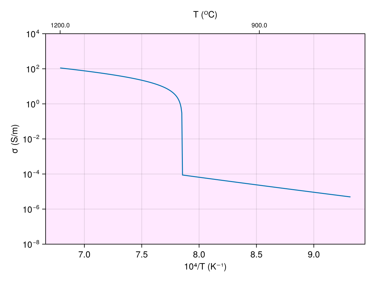

Please note that this is just one of the functions to calculate melt fractions, and you can define your own function and plug it in the fn_list defined above. In fact, fn_list can include multiple functions to better suit the needs, just keep in mind that these functions execute in the order they are placed in the list.

Let's take another example, this time around we use solidus_Hirschmann2000 to estimate solidus temperature. We also take into account the presence of volatiles and use get_Ch2o_m to partition the melt. This requires we also need a partition coefficient along with bulk water conc. Putting everything together, we have :

T = (1000:1600) .+ 273.0
P = 2.0
Ch2o = 1000.0
D = 0.005

ps_nt = (; T, P, Ch2o, D)

(T = 1273.0:1.0:1873.0, P = 2.0, Ch2o = 1000.0, D = 0.005)

Then we put together the fn_list. We first need to calculate the solidus temperature, then calculate the stable melt fraction and then partition water into olivine and melt.

fn_list = [solidus_Hirschmann2000, get_melt_fraction, get_Ch2o_m]
m_type = two_phase_modelType(Yoshino2009, Ni2011, HS1962_plus)
m = tune_rp_modelType(fn_list, m_type)

model = m(ps_nt)

and again forward response can be calculated as usual :

resp = forward(model, [])

Code for this figure

f = Figure()
ax = Axis(f[1, 1]; yscale=log10, xlabel="10⁴/T (K⁻¹)", ylabel="σ (S/m)",
    yticks=LogTicks(WilkinsonTicks(9; k_min=8)), backgroundcolor=(:magenta, 0.05))

xts = inv.([300, 600, 900, 1200, 1500] .+ 273.0) .* 1e4

ax2 = Axis(f[1, 1]; yscale=log10, xaxisposition=:top, yaxisposition=:right, xlabel="T (ᴼC)",
    xgridvisible=false, xtickformat=x -> string.(round.((1e4 ./ x) .- 273)),
    xticklabelsize=10, backgroundcolor=(:magenta, 0.05))
ax2.xticks = xts
hidespines!(ax2)
hideydecorations!(ax2)
linkyaxes!(ax, ax2)

logsig = resp.σ

lines!(ax, inv.(T) .* 1e4, 10 .^ logsig)
lines!(ax2, inv.(T) .* 1e4, 10 .^ logsig; alpha=0)

ylims!(ax, 1e-4, 1)
ylims!(ax2, 1e-4, 1e2)

┌ Warning: No strict ticks found
└ @ PlotUtils ~/.julia/packages/PlotUtils/HX80C/src/ticks.jl:194
┌ Warning: No strict ticks found
└ @ PlotUtils ~/.julia/packages/PlotUtils/HX80C/src/ticks.jl:194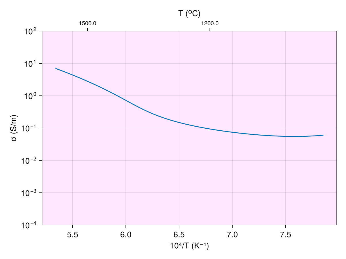

Custom functions

All the functions to be included in the list for tune_rp_model take a named tuple as an input and the same as output.