Solidus
Dry solidus
The dry solidus temperature can be obtained as a function of pressure P through solidus_Hirschmann2000 and solidus_Katz2003.
Code for this figure
julia
f = Figure()
ax1 = Axis(f[1, 1]; xlabel="solidus temp (K)", ylabel="depth (km)", backgroundcolor=(
    :magenta, 0.05))
ax1.yreversed = true

xtfn(x) = @. string(round((x - 5) / 30.2; digits=2))
ax2 = Axis(f[1, 1]; ylabel="Pressure (GPa)", yaxisposition=:right, xaxisposition=:top,
    xtickformat=xtfn, backgroundcolor=(:magenta, 0.05), yticks=WilkinsonTicks(6; k_min=5))
hidespines!(ax2)
hidexdecorations!(ax2)
linkxaxes!(ax1, ax2)

ax2.yreversed = true

z = 40:300
P = @. (z - 5) / 30.2
ps_nt = (; P)

sol_h = solidus_Hirschmann2000(ps_nt).T_solidus
sol_k = solidus_Katz2003(ps_nt).T_solidus

lines!(ax1, sol_h, z; label="Hirschmann2000")
lines!(ax1, sol_k, z; label="Katz2003")

f[1, 2] = Legend(f, ax1)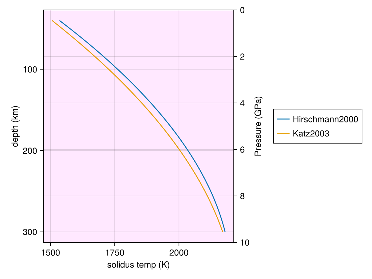
Effect of volatiles
Addition of volatiles lowers the solidus temperature facilitating more melting.
Water
Lowering of solidus due to water is available through ΔT_h2o_Katz2003 and ΔT_h2o_Blatter2022:
Code for this figure
julia
f = Figure()
ax1 = Axis(f[1, 1]; xlabel="solidus temp (K)", ylabel="depth (km)",
    backgroundcolor=(:magenta, 0.05), title="Katz2003")
ax1.yreversed = true

xtfn(x) = @. string(round((x - 5) / 30.2; digits=2))
ax2 = Axis(f[1, 1]; ylabel="Pressure (GPa)", yaxisposition=:right, xaxisposition=:top,
    xtickformat=xtfn, backgroundcolor=(:magenta, 0.05), yticks=WilkinsonTicks(6; k_min=5))
hidespines!(ax2)
hidexdecorations!(ax2)
linkxaxes!(ax1, ax2)
ax2.yreversed = true

ax3 = Axis(f[1, 2]; xlabel="solidus temp (K)", ylabel="depth (km)",
    backgroundcolor=(:magenta, 0.05), title="Blatter2022")
ax3.yreversed = true

xtfn(x) = @. string(round((x - 5) / 30.2; digits=2))
ax4 = Axis(f[1, 2]; ylabel="Pressure (GPa)", yaxisposition=:right, xaxisposition=:top,
    xtickformat=xtfn, backgroundcolor=(:magenta, 0.05), yticks=WilkinsonTicks(6; k_min=5))
hidespines!(ax4)
hidexdecorations!(ax4)
linkxaxes!(ax3, ax4)
ax4.yreversed = true

z = 40:300
P = @. (z - 5) / 30.2
ps_nt = (; P)

T_solidus = solidus_Hirschmann2000(ps_nt).T_solidus
Ch2o_m = inv(0.005) .* [0.01, 10.0, 100.0, 500.0, 1000.0, 2000.0]'
ps_nt = (; P, T_solidus, Ch2o_m)
T_wet_k = ΔT_h2o_Katz2003((; ps_nt..., T_solidus)).T_solidus

lines!(ax1, T_solidus, z; label="dry", color=:green, linewidth=6)
for i in eachindex(Ch2o_m)
    color_ = RGBf(1 - i / length(Ch2o_m), 0.0, i / length(Ch2o_m))
    w = Ch2o_m[i]
    lines!(ax1, T_wet_k[:, i], z; label="$(w/1f4)", color=color_)
end

T_wet_b = ΔT_h2o_Blatter2022((; ps_nt..., T_solidus)).T_solidus

lines!(ax3, T_solidus, z; label="dry", color=:green, linewidth=6)
for i in eachindex(Ch2o_m)
    color_ = RGBf(1 - i / length(Ch2o_m), 0.0, i / length(Ch2o_m))
    w = Ch2o_m[i]
    lines!(ax3, T_wet_b[:, i], z; label="$(w/1f4)", color=color_)
end

f[2, 1:2] = Legend(f, ax1, "melt water conc. (wt %)"; orientation=:horizontal)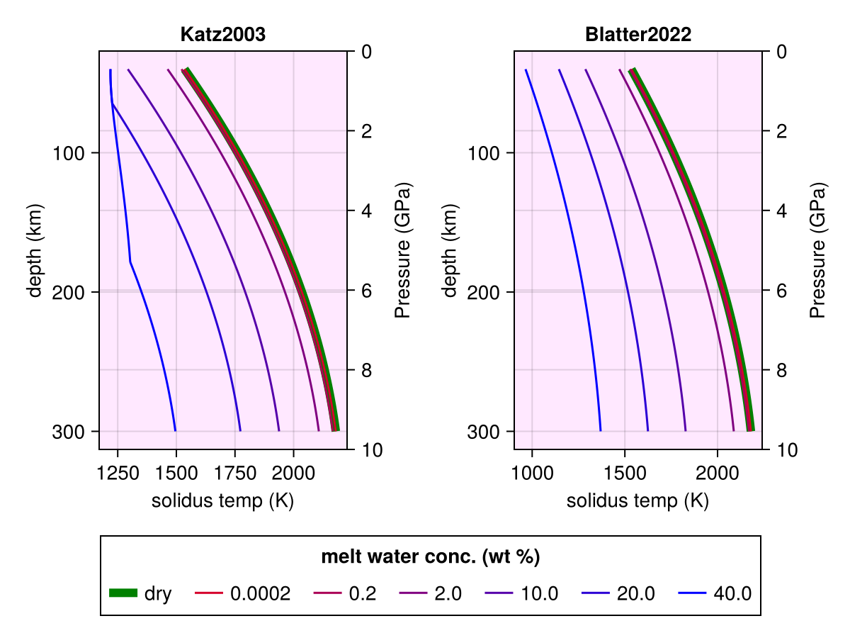
CO₂
Lowering of solidus due to CO₂ is available through ΔT_co2_Dasgupta2007 and ΔT_co2_Dasgupta2013:
Code for this figure
julia
f = Figure()
ax1 = Axis(f[1, 1]; xlabel="solidus temp (K)", ylabel="depth (km)",
    backgroundcolor=(:magenta, 0.05), title="Dasgupta2007")
ax1.yreversed = true

xtfn(x) = @. string(round((x - 5) / 30.2; digits=2))
ax2 = Axis(f[1, 1]; ylabel="Pressure (GPa)", yaxisposition=:right, xaxisposition=:top,
    xtickformat=xtfn, backgroundcolor=(:magenta, 0.05), yticks=WilkinsonTicks(6; k_min=5))
hidespines!(ax2)
hidexdecorations!(ax2)
linkxaxes!(ax1, ax2)
ax2.yreversed = true

ax3 = Axis(f[1, 2]; xlabel="solidus temp (K)", ylabel="depth (km)",
    backgroundcolor=(:magenta, 0.05), title="Dasgupta2013")
ax3.yreversed = true

xtfn(x) = @. string(round((x - 5) / 30.2; digits=2))
ax4 = Axis(f[1, 2]; ylabel="Pressure (GPa)", yaxisposition=:right, xaxisposition=:top,
    xtickformat=xtfn, backgroundcolor=(:magenta, 0.05), yticks=WilkinsonTicks(6; k_min=5))
hidespines!(ax4)
hidexdecorations!(ax4)
linkxaxes!(ax3, ax4)
ax4.yreversed = true

z = 40:300
P = @. (z - 5) / 30.2
ps_nt = (; P)

T_solidus = solidus_Hirschmann2000(ps_nt).T_solidus
Cco2_m = 1e4 .* [0.01, 1.0, 10.0, 30.0, 50.0]'
ps_nt = (; P, T_solidus, Cco2_m)
T_wet_k = ΔT_co2_Dasgupta2007((; ps_nt..., T_solidus)).T_solidus

lines!(ax1, T_solidus, z; label="dry", color=:green, linewidth=6)
for i in eachindex(Cco2_m)
    color_ = RGBf(1 - i / length(Cco2_m), 0.0, i / length(Cco2_m))
    w = Cco2_m[i]
    lines!(ax1, T_wet_k[:, i], z; label="$(w/1f4)", color=color_)
end

T_wet_b = ΔT_co2_Dasgupta2013((; ps_nt..., T_solidus)).T_solidus

lines!(ax3, T_solidus, z; label="dry", color=:green, linewidth=6)
for i in eachindex(Cco2_m)
    color_ = RGBf(1 - i / length(Cco2_m), 0.0, i / length(Cco2_m))
    w = Cco2_m[i]
    lines!(ax3, T_wet_b[:, i], z; label="$(w/1f4)", color=color_)
end

f[2, 1:2] = Legend(f, ax1, "melt CO₂ conc. (wt %)"; orientation=:horizontal)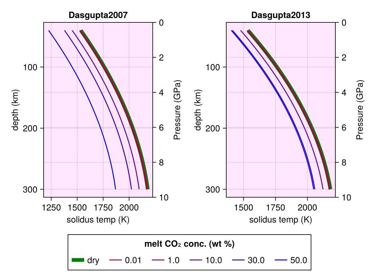
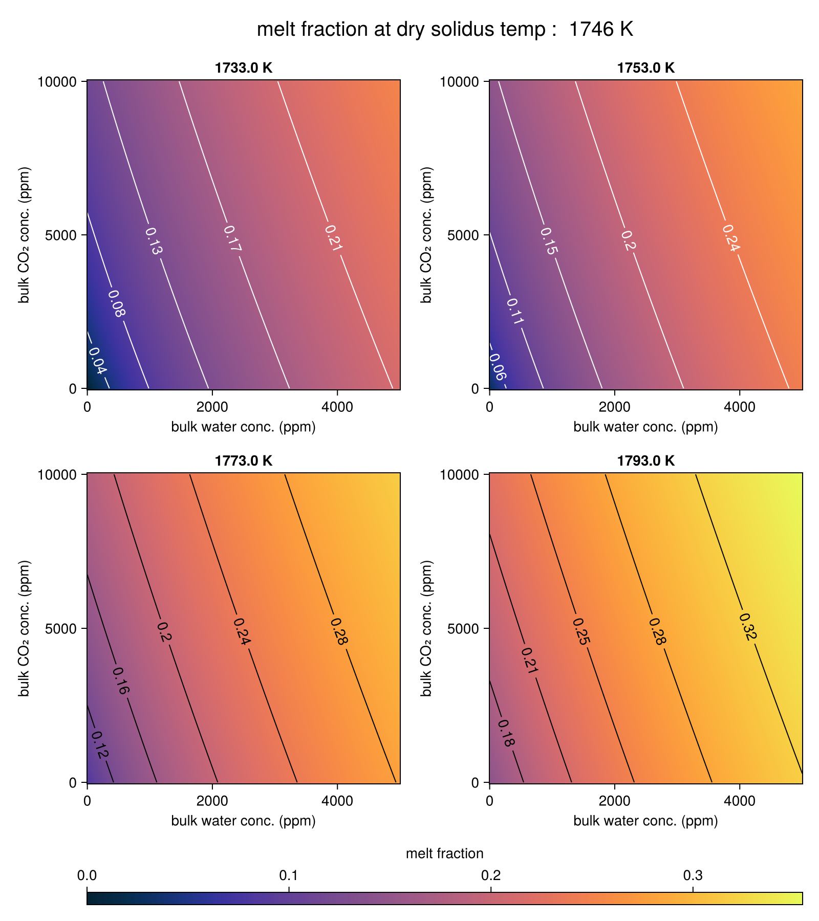
Stable melt fraction
Addition of volatiles lowers the solidus, generating more melt. The partitioning of volatiles into melt would, however, require knowing about the melt fraction beforehand. We, therefore, follow Blatter, et al., 2022 to estimate the amount of thermodynamically stable melt using get_melt_fraction.
Code for this figure
julia
P = 3.0
T_solidus = solidus_Hirschmann2000((; P)).T_solidus
T = [1460, 1480, 1500, 1520] .+ 273.0
D = 0.0093
Ch2o = reshape(collect(0.0:10:5000.0), 1, :)
Cco2 = reshape(collect(0.0:100:10000.0), 1, 1, :)

ps_nt = (; P, T, T_solidus, Ch2o, Cco2, D)
ϕ = get_melt_fraction(ps_nt).ϕ;
size(ϕ)

fig = Figure(; size=(800, 900))
ax1 = Axis(fig[1, 1]; xlabel="bulk water conc. (ppm)", ylabel="bulk CO₂ conc. (ppm)", title="$(T[1]) K")
ax2 = Axis(fig[1, 2]; xlabel="bulk water conc. (ppm)", ylabel="bulk CO₂ conc. (ppm)", title="$(T[2]) K")
ax3 = Axis(fig[2, 1]; xlabel="bulk water conc. (ppm)", ylabel="bulk CO₂ conc. (ppm)", title="$(T[3]) K")
ax4 = Axis(fig[2, 2]; xlabel="bulk water conc. (ppm)", ylabel="bulk CO₂ conc. (ppm)", title="$(T[4]) K")

crange = extrema(ϕ)
cmap = :thermal
heatmap!(ax1, vec(Ch2o), vec(Cco2), ϕ[1, :, :]; colorrange=crange, colormap=cmap)
contour!(ax1, vec(Ch2o), vec(Cco2), ϕ[1, :, :]; labels=true, color=:white, labelsize=14)
heatmap!(ax2, vec(Ch2o), vec(Cco2), ϕ[2, :, :]; colorrange=crange, colormap=cmap)
contour!(ax2, vec(Ch2o), vec(Cco2), ϕ[2, :, :]; labels=true, color=:white, labelsize=14)
heatmap!(ax3, vec(Ch2o), vec(Cco2), ϕ[3, :, :]; colorrange=crange, colormap=cmap)
contour!(ax3, vec(Ch2o), vec(Cco2), ϕ[3, :, :]; labels=true, color=:black, labelsize=14)
h = heatmap!(ax4, vec(Ch2o), vec(Cco2), ϕ[4, :, :]; colorrange=crange, colormap=cmap)
contour!(ax4, vec(Ch2o), vec(Cco2), ϕ[4, :, :]; labels=true, color=:black, labelsize=14)
Colorbar(fig[3, :], h; vertical=false, label="melt fraction")
Label(fig[0, :], "melt fraction at dry solidus temp :  $(Int(round(T_solidus))) K"; fontsize=20)