Visualization

We make use of Makie.jl to generate images. This allows us to be more flexible with and also generate more fancy figures.

Here, we want to give a slightly detailed outlook on generating figures. Makie.jl provides multiple backends to generate graphics. We use CairoMakie because it uses CPUs and is compatible with most machines. There is also GLMakie which makes use of GPUs, and the same functions should work with any backend.

Using Makie

Makie.jl works around three objects : scene, figure and axis. Of these three, scene is mostly useful for 3D rendering, which, while is a nice feature, is not really useful for us. We, therefore, make use of the latter two.

While a more interested reader is encouraged to explore the Makie.jl documentation, here we suffice by saying that a figure is the whole figure, containing multiple axis objects. Each axis can contain a plot, colorbar, legend, etc. Therefore, we advised that while creating legends, use another axis. This allows more control.

For the purpose of this tutorial, know that when you call a plotting function, it returns a figure and all the axis in the figure. You must have guessed by now, but we want to make it slightly more explicit that most of the plotting happens on axis while figure is just a container around it to control the aspects (pun intended) of the figure. Therefore, when overlaying multiple plots on the same graph, we only need axis and not necessarily figure. All the mutating functions, therefore, ask for axis.

If you want to make an empty figure, just call:

using CairoMakie
f = Figure(; size=(200, 200))
f

We now have the container. Time to add an axis:

ax = Axis(f[1, 1])
f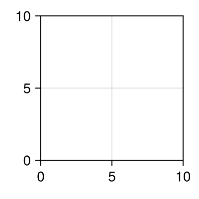

Let's add another

ax1 = Axis(f[2, 1])
f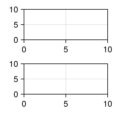

and another...

ax2 = Axis(f[2, 2])
f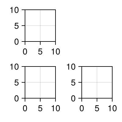

Notice the arrangement of axes according to the indices passed for f in Axis. This allows us to create more fanciful layouts:

f = Figure(; size=(200, 200))
ax1 = Axis(f[1:2, 1])
ax2 = Axis(f[1:2, 2])
ax3 = Axis(f[3, 1])
ax4 = Axis(f[3, 2])
ax5 = Axis(f[1:3, 3])
f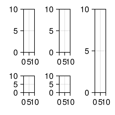

The usage will become more apparent with the following example:

Plotting models

Let's say you have a model defined as :

arr1 = randn(100)
arr2 = randn(100)

100-element Vector{Float64}:
 -0.8437593385659486
 -1.560846746072158
 -0.01972736702273779
 -0.35635689583392666
  0.9850776226174748
  1.854584697406609
 -0.9964508926468321
 -0.6306965932211727
  1.412180135050873
  2.5386969033381
  ⋮
 -0.7242191942768508
  1.8967517634281958
 -0.23148180611012484
  0.17709959897105454
 -0.5253628666828345
  0.19477223009961087
 -0.24632139640854644
  1.3233126452731867
 -0.073131051722828

Now, we plot the model with :

f, ax = scatter(arr1, arr2)
f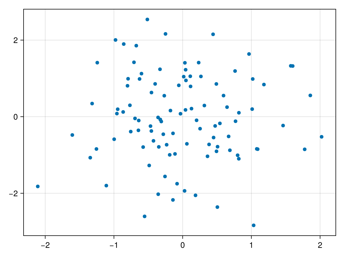

See how the plot_model function returns a figure and an axis. If we want to overlay another plot, we make use of mutating functions, the ones ending in a !

arr3 = arr1 .^ 2
lines!(arr1, arr3)

Makie.Lines{Tuple{Vector{GeometryBasics.Point{2, Float64}}}}

We only needed to pass ax to plot on the same axis. This might also seem a bit intuitive as well. At this point, we want to encourage creating empty figure beforehand and then always using mutating functions. This gives us more control on how the axes are arranged among other stuff. Here's an example to make things clear.

x = 2π .* (0:0.01:1)
y1 = @. sin(x)
y2 = @. cos(x)

f = Figure(; size=(200, 200)) # creating empty figure
ax = Axis(f[1, 1])

lines!(ax, x, y1)
lines!(ax, x, y2)
f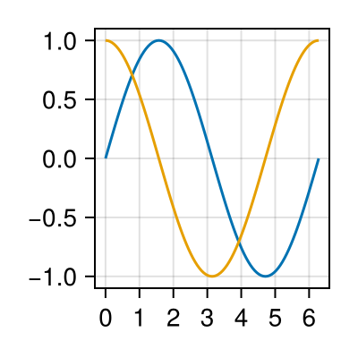

Notice how the above plots did not have legends. Note that legends are another axis.

x = 2π .* (0:0.01:1)
y1 = @. sin(x)
y2 = @. cos(x)

f = Figure(; size=(200, 200)) # creating empty figure
ax = Axis(f[1, 1])

lines!(ax, x, y1; label="sin(x)")
lines!(ax, x, y2; label="cos(x)")

Legend(f[1, 2], ax)
f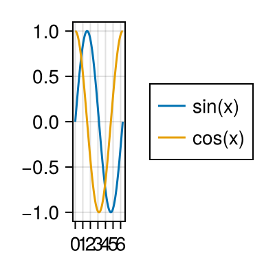

Concluding remarks

This tutorial is to give you a walkthrough of how Makie works in our context. Most other plotting functions in the package follow the same style. Makie.jl has a number of keyword arguments to customize the plots. Do checkout the respective documentations.