Elasticity models
Anharmonic scaling
Porosity.anharmonic Type
anharmonic(T, P, ρ)Calculate unrelaxed elastic bulk moduli, shear moduli, Vp and Vs using anharmonic scaling
Arguments
- `T` : Temperature of the rock (K)
- `P` : Pressure (GPa)
- `ρ` : Density of the rock (kg/m³)
Keyword Arguments
- `params` : Various coefficients required for calculation.
Available options are
    - `params_anharmonic.Isaak1992`
    - `params_anharmonic.Cammarono2003`
Defaults to the ones provided by Isaak (1992), check references.
To investigate coefficients, call `default_params(Val{anharmonic}())`.
To modify coefficients, check the relevant documentation page.
Usage
julia> T = collect(1273.0f0:40:1473.0f0);

julia> P = 2 .+ zero(T);

julia> ρ = collect(3300.0f0:200.0f0:4300.0f0);

julia> model = anharmonic(T, P, ρ)
Model : anharmonic
Temperature (K) : Float32[1273.0, 1313.0, 1353.0, 1393.0, 1433.0, 1473.0]
Pressure (GPa) : Float32[2.0, 2.0, 2.0, 2.0, 2.0, 2.0]
Density (kg/m³) : Float32[3300.0, 3500.0, 3700.0, 3900.0, 4100.0, 4300.0]

julia> forward(model, [])
Rock physics Response : RockphyElastic
Elastic shear modulus (Pa) : Float32[7.136702f10, 7.082302f10, 7.027902f10, 6.9735014f10, 6.919102f10, 6.864702f10]
Elastic bulk modulus (Pa) : Float32[1.1894502f11, 1.18038364f11, 1.1713171f11, 1.1622502f11, 1.1531837f11, 1.1441169f11]
Elastic P-wave velocity (m/s) : Float32[8054.7563, 7791.3696, 7548.708, 7324.0913, 7115.3057, 6920.496]
Elastic S-wave velocity (m/s) : Float32[4650.416, 4498.3496, 4358.2485, 4228.5664, 4108.0234, 3995.5503]
References
Cammarano et al. (2003), "Inferring upper-mantle temperatures from seismic velocities", Physics of the Earth and Planetary Interiors, Volume 138, Issues 3–4, https://doi.org/10.1016/S0031-9201(03)00156-0
Isaak, D. G. (1992), "High‐temperature elasticity of iron‐bearing olivines", J. Geophys. Res., 97( B2), 1871– 1885, https://doi.org/10.1029/91JB02675
The distribution with temperature looks like (assuming increase in density is not due to increase in pressure) at 2 GPa pressure:
Code for this figure
f = Figure(; size=(700, 700))

T = (600:1600) .+ 273.0
P = 2.0
ρ = [2700, 2900, 3100, 3300]'
m = anharmonic(T, P, ρ)
resp = forward(m, []);

resp_fields = [:K, :G, :Vp, :Vs]
units = ["GPa", "GPa", "km/s", "km/s"]

ax_coords = [(1, 1), (1, 2), (2, 1), (2, 2)]
for i in eachindex(resp_fields)
    ax = Axis(f[ax_coords[i]...]; xlabel="10⁴/T (K⁻¹)",
        ylabel=string(resp_fields[i]) * " ($(units[i]))",
        yticks=LogTicks(WilkinsonTicks(6; k_min=5)), backgroundcolor=(:magenta, 0.052))

    xts = inv.([600, 800, 1000, 1200, 1600] .+ 273.0) .* 1e4

    ax2 = Axis(
        f[ax_coords[i]...]; xaxisposition=:top, yaxisposition=:right, xlabel="T (ᴼC)",
        xgridvisible=false, xtickformat=x -> string.(round.((1e4 ./ x) .- 273)),
        xticklabelsize=8, backgroundcolor=(:magenta, 0.05))
    ax2.xticks = xts
    hidespines!(ax2)
    hideydecorations!(ax2)
    linkyaxes!(ax, ax2)

    for j in axes(getfield(resp, resp_fields[i]), 2)
        d = ρ[j]
        r_ = getfield(resp, resp_fields[i])
        lines!(ax, inv.(T) .* 1e4, r_[:, j]; label="$d")
        lines!(ax2, inv.(T) .* 1e4, r_[:, j]; alpha=0)
    end
end
f[3, 1:2] = Legend(f, f.content[end - 1], "density (kg/m³)"; orientation=:horizontal)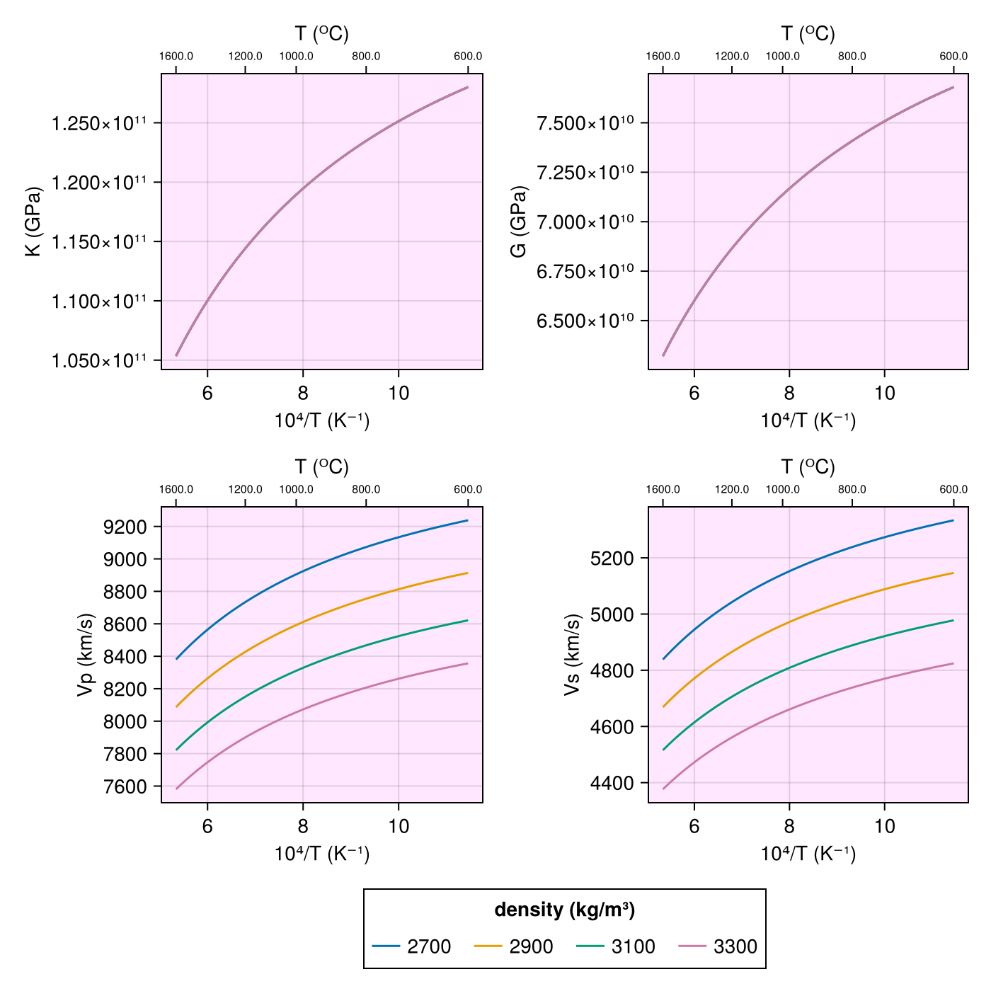
Anharmonic (porous) scaling
Porosity.anharmonic Type
anharmonic(T, P, ρ)Calculate unrelaxed elastic bulk moduli, shear moduli, Vp and Vs using anharmonic scaling
Arguments
- `T` : Temperature of the rock (K)
- `P` : Pressure (GPa)
- `ρ` : Density of the rock (kg/m³)
Keyword Arguments
- `params` : Various coefficients required for calculation.
Available options are
    - `params_anharmonic.Isaak1992`
    - `params_anharmonic.Cammarono2003`
Defaults to the ones provided by Isaak (1992), check references.
To investigate coefficients, call `default_params(Val{anharmonic}())`.
To modify coefficients, check the relevant documentation page.
Usage
julia> T = collect(1273.0f0:40:1473.0f0);

julia> P = 2 .+ zero(T);

julia> ρ = collect(3300.0f0:200.0f0:4300.0f0);

julia> model = anharmonic(T, P, ρ)
Model : anharmonic
Temperature (K) : Float32[1273.0, 1313.0, 1353.0, 1393.0, 1433.0, 1473.0]
Pressure (GPa) : Float32[2.0, 2.0, 2.0, 2.0, 2.0, 2.0]
Density (kg/m³) : Float32[3300.0, 3500.0, 3700.0, 3900.0, 4100.0, 4300.0]

julia> forward(model, [])
Rock physics Response : RockphyElastic
Elastic shear modulus (Pa) : Float32[7.136702f10, 7.082302f10, 7.027902f10, 6.9735014f10, 6.919102f10, 6.864702f10]
Elastic bulk modulus (Pa) : Float32[1.1894502f11, 1.18038364f11, 1.1713171f11, 1.1622502f11, 1.1531837f11, 1.1441169f11]
Elastic P-wave velocity (m/s) : Float32[8054.7563, 7791.3696, 7548.708, 7324.0913, 7115.3057, 6920.496]
Elastic S-wave velocity (m/s) : Float32[4650.416, 4498.3496, 4358.2485, 4228.5664, 4108.0234, 3995.5503]
References
Cammarano et al. (2003), "Inferring upper-mantle temperatures from seismic velocities", Physics of the Earth and Planetary Interiors, Volume 138, Issues 3–4, https://doi.org/10.1016/S0031-9201(03)00156-0
Isaak, D. G. (1992), "High‐temperature elasticity of iron‐bearing olivines", J. Geophys. Res., 97( B2), 1871– 1885, https://doi.org/10.1029/91JB02675
The distribution with temperature looks like (assuming increase in porosity is not related to pressure (2 GPa) or density (3000 kg/m³)) :
Code for this figure
f = Figure(; size=(700, 700))

T = (600:1600) .+ 273.0
P = 2.0
ρ = 3300.0
ϕ = [0.01, 0.03, 0.1, 0.3]'
m = anharmonic_poro(T, P, ρ, ϕ)
resp = forward(m, []);

resp_fields = [:K, :G, :Vp, :Vs]
units = ["GPa", "GPa", "km/s", "km/s"]

ax_coords = [(1, 1), (1, 2), (2, 1), (2, 2)]
for i in eachindex(resp_fields)
    ax = Axis(f[ax_coords[i]...]; xlabel="10⁴/T (K⁻¹)",
        ylabel=string(resp_fields[i]) * " ($(units[i]))",
        yticks=LogTicks(WilkinsonTicks(6; k_min=5)), backgroundcolor=(:magenta, 0.052))

    xts = inv.([600, 800, 1000, 1200, 1600] .+ 273.0) .* 1e4

    ax2 = Axis(
        f[ax_coords[i]...]; xaxisposition=:top, yaxisposition=:right, xlabel="T (ᴼC)",
        xgridvisible=false, xtickformat=x -> string.(round.((1e4 ./ x) .- 273)),
        xticklabelsize=8, backgroundcolor=(:magenta, 0.05))
    ax2.xticks = xts
    hidespines!(ax2)
    hideydecorations!(ax2)
    linkyaxes!(ax, ax2)

    for j in axes(getfield(resp, resp_fields[i]), 2)
        d = ϕ[j]
        r_ = getfield(resp, resp_fields[i])
        lines!(ax, inv.(T) .* 1e4, r_[:, j]; label="$d")
        lines!(ax2, inv.(T) .* 1e4, r_[:, j]; alpha=0)
    end
end
f[3, 1:2] = Legend(f, f.content[end - 1], "Porosity"; orientation=:horizontal)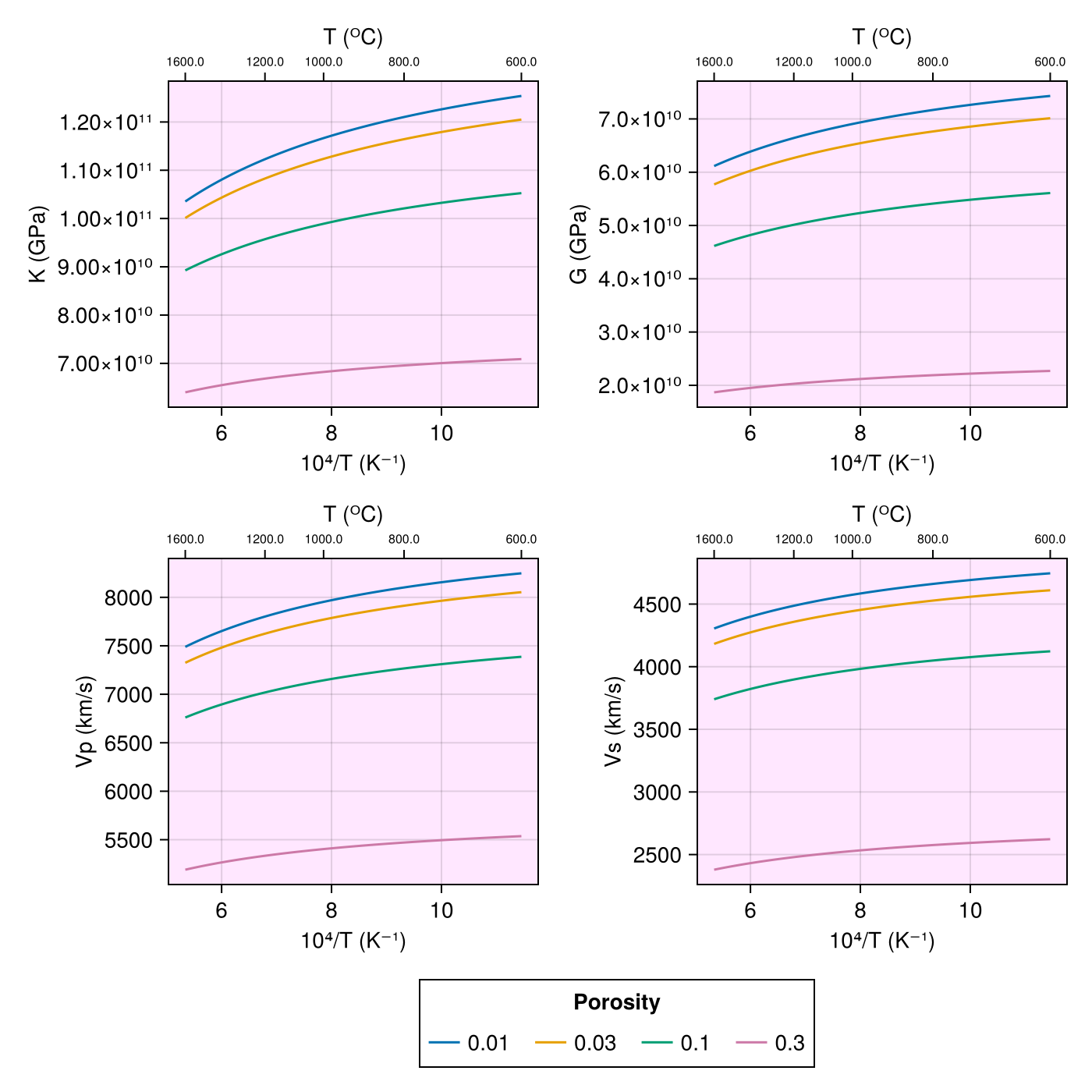
The distribution with temperature at constant porosity (0.1) (assuming increase in density is not related to pressure (2 GPa)) :
Code for this figure
f = Figure(; size=(700, 700))

T = (600:1600) .+ 273.0
P = 2.0
ρ = [2700, 2900, 3100, 3300]'
ϕ = 0.1
m = anharmonic_poro(T, P, ρ, ϕ)
resp = forward(m, []);

resp_fields = [:K, :G, :Vp, :Vs]
units = ["GPa", "GPa", "km/s", "km/s"]

ax_coords = [(1, 1), (1, 2), (2, 1), (2, 2)]
for i in eachindex(resp_fields)
    ax = Axis(f[ax_coords[i]...]; xlabel="10⁴/T (K⁻¹)",
        ylabel=string(resp_fields[i]) * " ($(units[i]))",
        yticks=LogTicks(WilkinsonTicks(6; k_min=5)), backgroundcolor=(:magenta, 0.052))

    xts = inv.([600, 800, 1000, 1200, 1600] .+ 273.0) .* 1e4

    ax2 = Axis(
        f[ax_coords[i]...]; xaxisposition=:top, yaxisposition=:right, xlabel="T (ᴼC)",
        xgridvisible=false, xtickformat=x -> string.(round.((1e4 ./ x) .- 273)),
        xticklabelsize=8, backgroundcolor=(:magenta, 0.05))
    ax2.xticks = xts
    hidespines!(ax2)
    hideydecorations!(ax2)
    linkyaxes!(ax, ax2)

    for j in axes(getfield(resp, resp_fields[i]), 2)
        d = ρ[j]
        r_ = getfield(resp, resp_fields[i])
        lines!(ax, inv.(T) .* 1e4, r_[:, j]; label="$d")
        lines!(ax2, inv.(T) .* 1e4, r_[:, j]; alpha=0)
    end
end
f[3, 1:2] = Legend(f, f.content[end - 1], "Porosity"; orientation=:horizontal)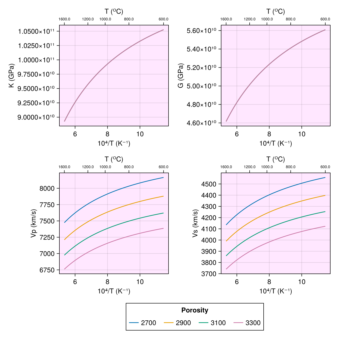
SLB2005
Porosity.SLB2005 Type
SLB2005(T, P)Calculate upper mantle shear velocity using Stixrude and Lithgow‐Bertelloni (2005) fit of upper mantle Vs.
Warning
Note that the other parameters (elastic moudli and Vp) are populated with zeros.
Arguments
- `T` : Temperature of the rock (K)
- `P` : Pressure (GPa)
Keyword Arguments
- `params` : Various coefficients required for calculation.
Does not have any coefficients that can be changed and hence is an empty `NamedTuple`
Usage
julia> T = collect(1273.0f0:40:1473.0f0);

julia> P = 2 .+ zero(T);

julia> model = SLB2005(T, P)
Model : SLB2005
Temperature (K) : Float32[1273.0, 1313.0, 1353.0, 1393.0, 1433.0, 1473.0]
Pressure (GPa) : Float32[2.0, 2.0, 2.0, 2.0, 2.0, 2.0]

julia> forward(model, [])
Rock physics Response : RockphyElastic
Elastic shear modulus (Pa) : Float32[0.0, 0.0, 0.0, 0.0, 0.0, 0.0]
Elastic bulk modulus (Pa) : Float32[0.0, 0.0, 0.0, 0.0, 0.0, 0.0]
Elastic P-wave velocity (m/s) : Float32[0.0, 0.0, 0.0, 0.0, 0.0, 0.0]
Elastic S-wave velocity (m/s) : [4478.205990493298, 4463.085990846157, 4447.965991199017, 4432.845991551876, 4417.725991904736, 4402.605992257595]
References
- Stixrude and Lithgow‐Bertelloni (2005), "Mineralogy and elasticity of the oceanic upper mantle: Origin of the low‐velocity zone." JGR 110.B3, https://doi.org/10.1029/2004JB002965
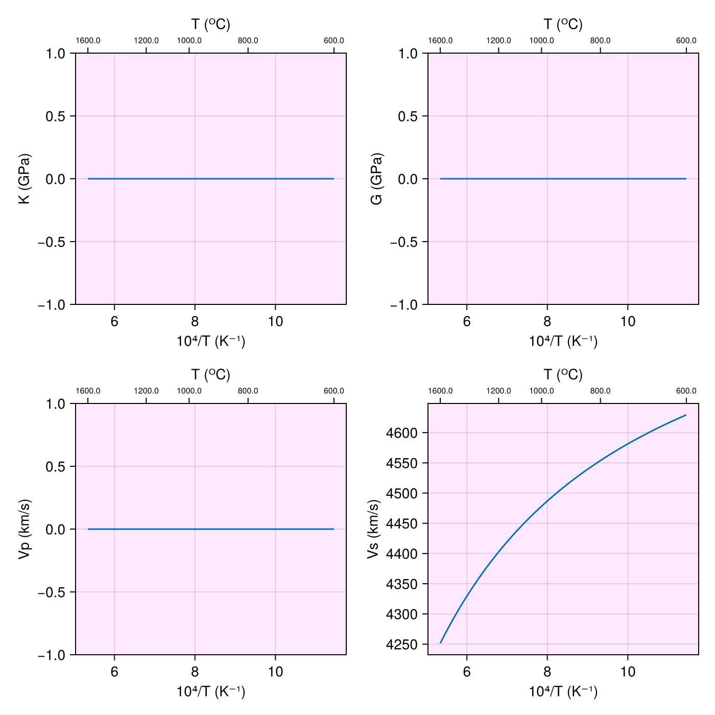
The distribution with temperature looks like (assuming increase in density is not due to increase in pressure) at 2 GPa pressure:
Note
Note that the K, G and Vp fields are populated with zeros.
Code for this figure
f = Figure(; size=(700, 700))

T = (600:1600) .+ 273.0
P = 2.0
m = SLB2005(T, P)
resp = forward(m, []);

resp_fields = [:K, :G, :Vp, :Vs]
units = ["GPa", "GPa", "km/s", "km/s"]

ax_coords = [(1, 1), (1, 2), (2, 1), (2, 2)]
for i in eachindex(resp_fields)
    ax = Axis(f[ax_coords[i]...]; xlabel="10⁴/T (K⁻¹)",
        ylabel=string(resp_fields[i]) * " ($(units[i]))",
        yticks=LogTicks(WilkinsonTicks(6; k_min=5)), backgroundcolor=(:magenta, 0.052))

    xts = inv.([600, 800, 1000, 1200, 1600] .+ 273.0) .* 1e4

    ax2 = Axis(
        f[ax_coords[i]...]; xaxisposition=:top, yaxisposition=:right, xlabel="T (ᴼC)",
        xgridvisible=false, xtickformat=x -> string.(round.((1e4 ./ x) .- 273)),
        xticklabelsize=8, backgroundcolor=(:magenta, 0.05))
    ax2.xticks = xts
    hidespines!(ax2)
    hideydecorations!(ax2)
    linkyaxes!(ax, ax2)

    r_ = getfield(resp, resp_fields[i])
    lines!(ax, inv.(T) .* 1e4, r_)
    lines!(ax2, inv.(T) .* 1e4, r_; alpha=0)
end