Conductivity models

Minerals

SEO3

julia

SEO3(T)

Electrical conductivity model for olivine dependent on temperature.

Arguments

julia

- `T` : Temperature of olivine (in K)

Usage

julia

julia> model = SEO3(1000 + 273.0)
Model : SEO3
Temperature (K) : 1273.0

julia> forward(model, [])
Rock physics Response : RockphyCond
log₁₀ conductivity (S/m) : -4.0571856119909375

References

Constable, S (2006), "SEO3: A new model of olivine electrical conductivity", Geophysical Journal International, Volume 166, Issue 1, July 2006, Pages 435–437, https://doi.org/10.1111/j.1365-246X.2006.03041.x

source

The distribution with temperature looks like (compare with fig. 1B of Constable, 2003):

Code for this figure

julia

f = Figure()
ax = Axis(f[1, 1]; yscale=log10, xlabel="10⁴/T (K⁻¹)", ylabel="σ (S/m)",
    yticks=LogTicks(WilkinsonTicks(6; k_min=5)), backgroundcolor=(:magenta, 0.05))

xts = inv.([700, 900, 1100, 1300, 1500] .+ 273.0) .* 1e4

ax2 = Axis(f[1, 1]; yscale=log10, xaxisposition=:top, yaxisposition=:right, xlabel="T (ᴼC)",
    xgridvisible=false, xtickformat=x -> string.(round.((1e4 ./ x) .- 273)),
    xticklabelsize=10, backgroundcolor=(:magenta, 0.05))
ax2.xticks = xts
hidespines!(ax2)
hideydecorations!(ax2)
linkyaxes!(ax, ax2)

T = (700:1600) .+ 273.0
m = SEO3(T)
logsig = forward(m, []).σ

lines!(ax, inv.(T) .* 1e4, 10 .^ logsig)
lines!(ax2, inv.(T) .* 1e4, 10 .^ logsig; alpha=0)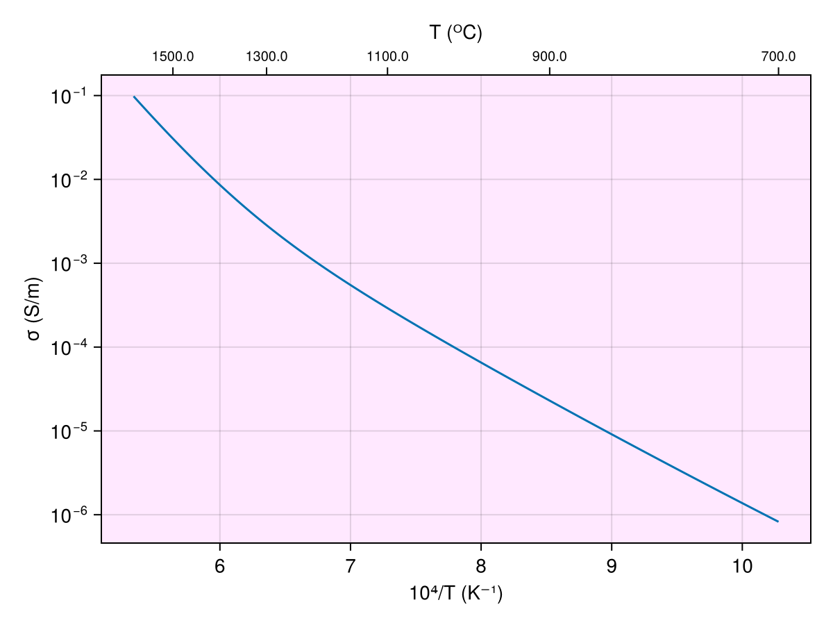

Wang2006

Porosity.Wang2006 Type

julia

Wang2006(T, Ch2o_ol)

Electrical conductivity model for olivine dependent on temperature and water concentration.

Arguments

T : Temperature of olivine (in K)
Ch2o_ol : water concentration in olivine (in ppm)

Usage

julia

julia> model = Wang2006(1000 + 273.0, 2e4)
Model : Wang2006
Temperature (K) : 1273.0
Water concentration in olivine (ppm) : 20000.0

julia> log_cond = forward(model, [])
Rock physics Response : RockphyCond
log₁₀ conductivity (S/m) : -0.383209519477097

References

Wang, D., Mookherjee, M., Xu, Y. et al. (2006), "The effect of water on the electrical conductivity of olivine", Nature 443, 977–980 (2006), doi: https://doi.org/10.1038/nature05256

source

The distribution with temperature looks like (compare with fig. 2a of Wang et al., 2006):

Code for this figure

julia

f = Figure()
ax = Axis(f[1, 1]; yscale=log10, xlabel="10⁴/T (K⁻¹)", ylabel="σ (S/m)",
    yticks=LogTicks(WilkinsonTicks(9; k_min=8)), backgroundcolor=(:magenta, 0.05))

xts = inv.([300, 600, 900, 1200, 1500] .+ 273.0) .* 1e4

ax2 = Axis(f[1, 1]; yscale=log10, xaxisposition=:top, yaxisposition=:right, xlabel="T (ᴼC)",
    xgridvisible=false, xtickformat=x -> string.(round.((1e4 ./ x) .- 273)),
    xticklabelsize=10, backgroundcolor=(:magenta, 0.05))
ax2.xticks = xts
hidespines!(ax2)
hideydecorations!(ax2)
linkyaxes!(ax, ax2)

T = (500:1400) .+ 273.0
Ch2o = [0.0, 0.01, 0.03, 0.1]' .* 1e4
m = Wang2006(T, Ch2o)
logsig = forward(m, []).σ

for i in eachindex(Ch2o)
    w = Ch2o[i]
    lines!(ax, inv.(T) .* 1e4, 10 .^ logsig[:, i]; label="$w")
    lines!(ax2, inv.(T) .* 1e4, 10 .^ logsig[:, i]; alpha=0)
end
ylims!(ax, 1e-8, 1)
ylims!(ax2, 1e-8, 1)
f[1, 2] = Legend(f, ax, "water conc. (ppm)")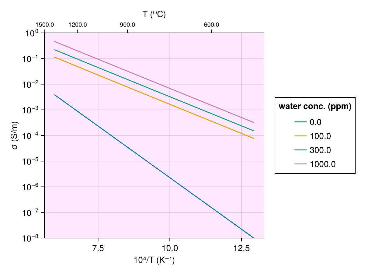

Yoshino2009

Porosity.Yoshino2009 Type

julia

Yoshino2009(T, Ch2o_ol)

Electrical conductivity model for olivine dependent on temperature and water concentration.

Arguments

T : Temperature of olivine (in K)
Ch2o_ol : water concentration in olivine (in ppm)

Usage

julia

julia> model = Yoshino2009(1000 + 273.0, 2e4)
Model : Yoshino2009
Temperature (K) : 1273.0
Water concentration in olivine (ppm) : 20000.0

julia> log_cond = forward(model, [])
Rock physics Response : RockphyCond
log₁₀ conductivity (S/m) : -0.6428765173222217

References

Takashi Yoshino, Takuya Matsuzaki, Anton Shatskiy, Tomoo Katsura (2009), "The effect of water on the electrical conductivity of olivine aggregates and its implications for the electrical structure of the upper mantle, Earth and Planetary Science Letters", Volume 288, Issues 1–2, 2009, Pages 291-300, ISSN 0012-821X, https://doi.org/10.1016/j.epsl.2009.09.032

source

The distribution with temperature looks like (compare with fig. 6 of Yoshino et al., 2009):

Code for this figure

julia

f = Figure()
ax = Axis(f[1, 1]; yscale=log10, xlabel="10⁴/T (K⁻¹)", ylabel="σ (S/m)",
    yticks=LogTicks(WilkinsonTicks(6; k_min=5)), backgroundcolor=(:magenta, 0.05))

xts = inv.([600, 800, 1000, 1200, 1400, 1600] .+ 273.0) .* 1e4

ax2 = Axis(f[1, 1]; yscale=log10, xaxisposition=:top, yaxisposition=:right, xlabel="T (ᴼC)",
    xgridvisible=false, xtickformat=x -> string.(round.((1e4 ./ x) .- 273)),
    xticklabelsize=8, backgroundcolor=(:magenta, 0.05))
ax2.xticks = xts
hidespines!(ax2)
hideydecorations!(ax2)
linkyaxes!(ax, ax2)

T = (600:1600) .+ 273.0
Ch2o = [0.0, 400, 600, 2000]'
m = Yoshino2009(T, Ch2o)
logsig = forward(m, []).σ

for i in eachindex(Ch2o)
    w = Ch2o[i]
    lines!(ax, inv.(T) .* 1e4, 10 .^ logsig[:, i]; label="$w")
    lines!(ax2, inv.(T) .* 1e4, 10 .^ logsig[:, i]; alpha=0)
end
ylims!(ax, 1e-7, 1)
ylims!(ax2, 1e-7, 1)
f[1, 2] = Legend(f, ax, "water conc. (ppm)")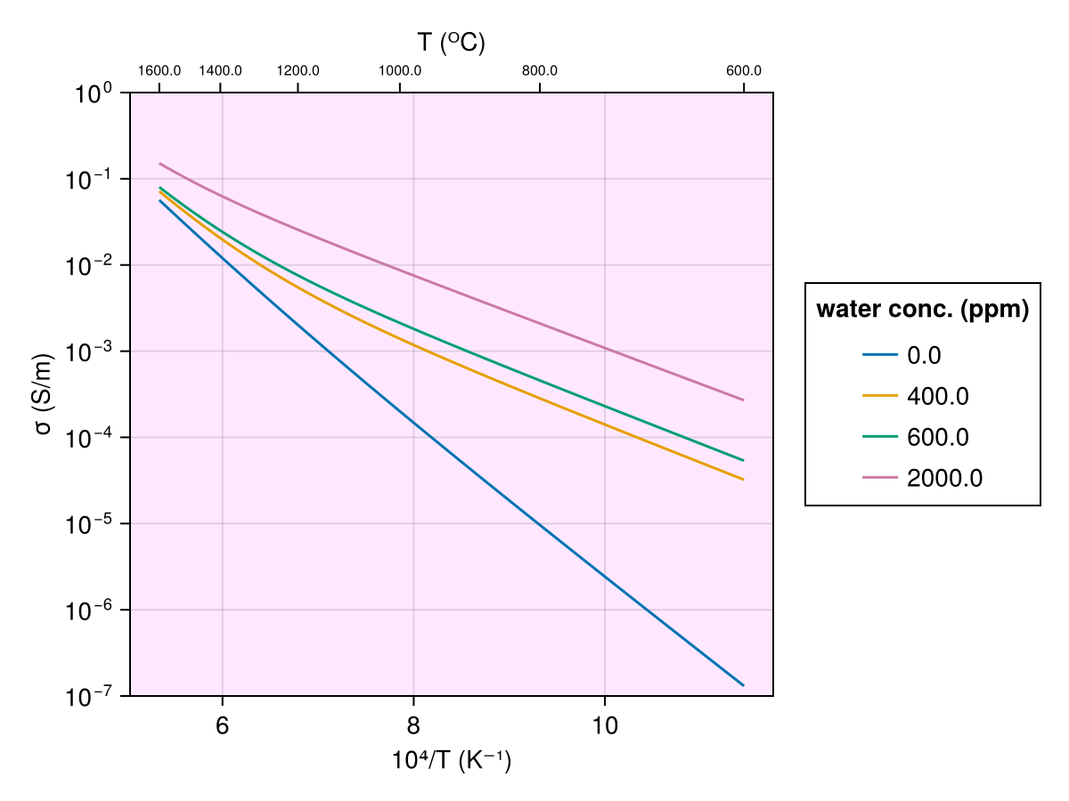

Poe2010

Porosity.Poe2010 Type

julia

Poe2010(T, Ch2o_ol)

Electrical conductivity model for olivine dependent on temperature and water concentration.

Arguments

T : Temperature of olivine (in K)
Ch2o_ol : water concentration in olivine (in ppm)

Usage

julia

julia> model = Poe2010(1000 + 273.0, 2e4)
Model : Poe2010
Temperature (K) : 1273.0
Water concentration in olivine (ppm) : 20000.0

julia> log_cond = forward(model, [])
Rock physics Response : RockphyCond
log₁₀ conductivity (S/m) : 3.4473300721921056

References

Brent T. Poe, Claudia Romano, Fabrizio Nestola, Joseph R. Smyth (2010), "Electrical conductivity anisotropy of dry and hydrous olivine at 8GPa", Physics of the Earth and Planetary Interiors,Volume 181, Issues 3–4, 2010, Pages 103-111, ISSN 0031-9201, https://doi.org/10.1016/j.pepi.2010.05.003.

source

The distribution with temperature looks like (compare with fig. 3 of Poe et al., 2010):

Code for this figure

julia

f = Figure()
ax = Axis(f[1, 1]; yscale=log10, xlabel="10⁴/T (K⁻¹)", ylabel="σ (S/m)",
    yticks=LogTicks(WilkinsonTicks(6; k_min=5)), backgroundcolor=(:magenta, 0.05))

xts = inv.([300, 600, 900, 1200, 1500] .+ 273.0) .* 1e4

ax2 = Axis(f[1, 1]; yscale=log10, xaxisposition=:top, yaxisposition=:right, xlabel="T (ᴼC)",
    xgridvisible=false, xtickformat=x -> string.(round.((1e4 ./ x) .- 273)),
    xticklabelsize=8, backgroundcolor=(:magenta, 0.05))
ax2.xticks = xts
hidespines!(ax2)
hideydecorations!(ax2)
linkyaxes!(ax, ax2)

T = (200:1600) .+ 273.0
Ch2o = [0.0, 400, 600, 2000]'
m = Poe2010(T, Ch2o)
logsig = forward(m, []).σ

for i in eachindex(Ch2o)
    w = Ch2o[i]
    lines!(ax, inv.(T) .* 1e4, 10 .^ logsig[:, i]; label="$w")
    lines!(ax2, inv.(T) .* 1e4, 10 .^ logsig[:, i]; alpha=0)
end
ylims!(ax, 1e-6, 10)
ylims!(ax2, 1e-6, 10)
f[1, 2] = Legend(f, ax, "water conc. (ppm)")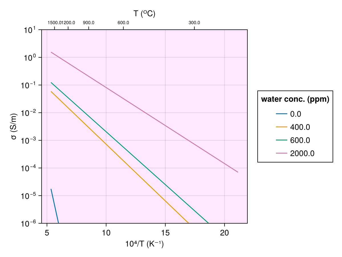

Jones2012

Porosity.Jones2012 Type

julia

Jones2012(T, Ch2o_ol)

Electrical conductivity model for olivine dependent on temperature and water concentration.

Arguments

T : Temperature of olivine (in K)
Ch2o_ol : water concentration in olivine (in ppm)

Usage

julia

julia> model = Jones2012(1000 + 273.0, 2e4)
Model : Jones2012
Temperature (K) : 1273.0
Water concentration in olivine (ppm) : 20000.0

julia> log_cond = forward(model, [])
Rock physics Response : RockphyCond
log₁₀ conductivity (S/m) : 0.15504093485137044

References

Jones, A. G., J. Fullea, R. L. Evans, and M. R. Muller (2012), "Water in cratonic lithosphere: Calibrating laboratory-determined models of electrical conductivity of mantle minerals using geophysical and petrological observations", Geochem. Geophys. Geosyst., 13, Q06010, doi:10.1029/2012GC004055.

source

The distribution with temperature looks like:

Code for this figure

julia

f = Figure()
ax = Axis(f[1, 1]; yscale=log10, xlabel="10⁴/T (K⁻¹)", ylabel="σ (S/m)",
    yticks=LogTicks(WilkinsonTicks(6; k_min=5)), backgroundcolor=(:magenta, 0.05))

xts = inv.([300, 600, 900, 1200, 1500] .+ 273.0) .* 1e4

ax2 = Axis(f[1, 1]; yscale=log10, xaxisposition=:top, yaxisposition=:right, xlabel="T (ᴼC)",
    xgridvisible=false, xtickformat=x -> string.(round.((1e4 ./ x) .- 273)),
    xticklabelsize=8, backgroundcolor=(:magenta, 0.05))
ax2.xticks = xts
hidespines!(ax2)
hideydecorations!(ax2)
linkyaxes!(ax, ax2)

T = (200:1600) .+ 273.0
Ch2o = [0.0, 400, 600, 2000]'
m = Jones2012(T, Ch2o)
logsig = forward(m, []).σ

for i in eachindex(Ch2o)
    w = Ch2o[i]
    lines!(ax, inv.(T) .* 1e4, 10 .^ logsig[:, i]; label="$w")
    lines!(ax2, inv.(T) .* 1e4, 10 .^ logsig[:, i]; alpha=0)
end
ylims!(ax, 1e-6, 10)
ylims!(ax2, 1e-6, 10)
f[1, 2] = Legend(f, ax, "water conc. (ppm)")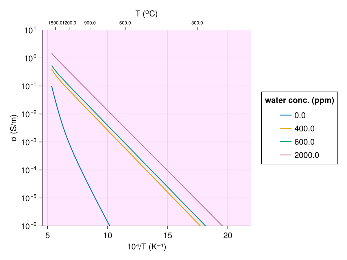

UHO2014

Porosity.UHO2014 Type

julia

UHO2014(T, Ch2o_ol)

Electrical conductivity model for olivine dependent on temperature and water concentration.

Arguments

T : Temperature of olivine (in K)
Ch2o_ol : water concentration in olivine (in ppm)

References

Gardés, E., F. Gaillard, and P. Tarits (2014), "Toward a unified hydrous olivine electrical conductivity law", Geochem. Geophys. Geosyst., 15, 4984–5000, doi:10.1002/2014GC005496.

Usage

julia

julia> model = UHO2014(1000 + 273.0, 2e4)
Model : UHO2014
Temperature (K) : 1273.0
Water concentration in olivine (ppm) : 20000.0

julia> log_cond = forward(model, [])
Rock physics Response : RockphyCond
log₁₀ conductivity (S/m) : 1.2727662435353444

source

The distribution with temperature looks like (compare with fig. 4 of Gardés et al., 2010):

Code for this figure

julia

f = Figure()
ax = Axis(f[1, 1]; yscale=log10, xlabel="10⁴/T (K⁻¹)", ylabel="σ (S/m)",
    yticks=LogTicks(WilkinsonTicks(6; k_min=5)), backgroundcolor=(:magenta, 0.05))

xts = inv.([600, 800, 1000, 1200, 1400, 1600] .+ 273.0) .* 1e4

ax2 = Axis(f[1, 1]; yscale=log10, xaxisposition=:top, yaxisposition=:right, xlabel="T (ᴼC)",
    xgridvisible=false, xtickformat=x -> string.(round.((1e4 ./ x) .- 273)),
    xticklabelsize=8, backgroundcolor=(:magenta, 0.05))
ax2.xticks = xts
hidespines!(ax2)
hideydecorations!(ax2)
linkyaxes!(ax, ax2)

T = (600:1600) .+ 273.0
Ch2o = [0.0, 400, 600, 2000]'
m = Jones2012(T, Ch2o)
logsig = forward(m, []).σ

for i in eachindex(Ch2o)
    w = Ch2o[i]
    lines!(ax, inv.(T) .* 1e4, 10 .^ logsig[:, i]; label="$w")
    lines!(ax2, inv.(T) .* 1e4, 10 .^ logsig[:, i]; alpha=0)
end
ylims!(ax, 1e-10, 10)
ylims!(ax2, 1e-10, 10)
f[1, 2] = Legend(f, ax, "water conc. (ppm)")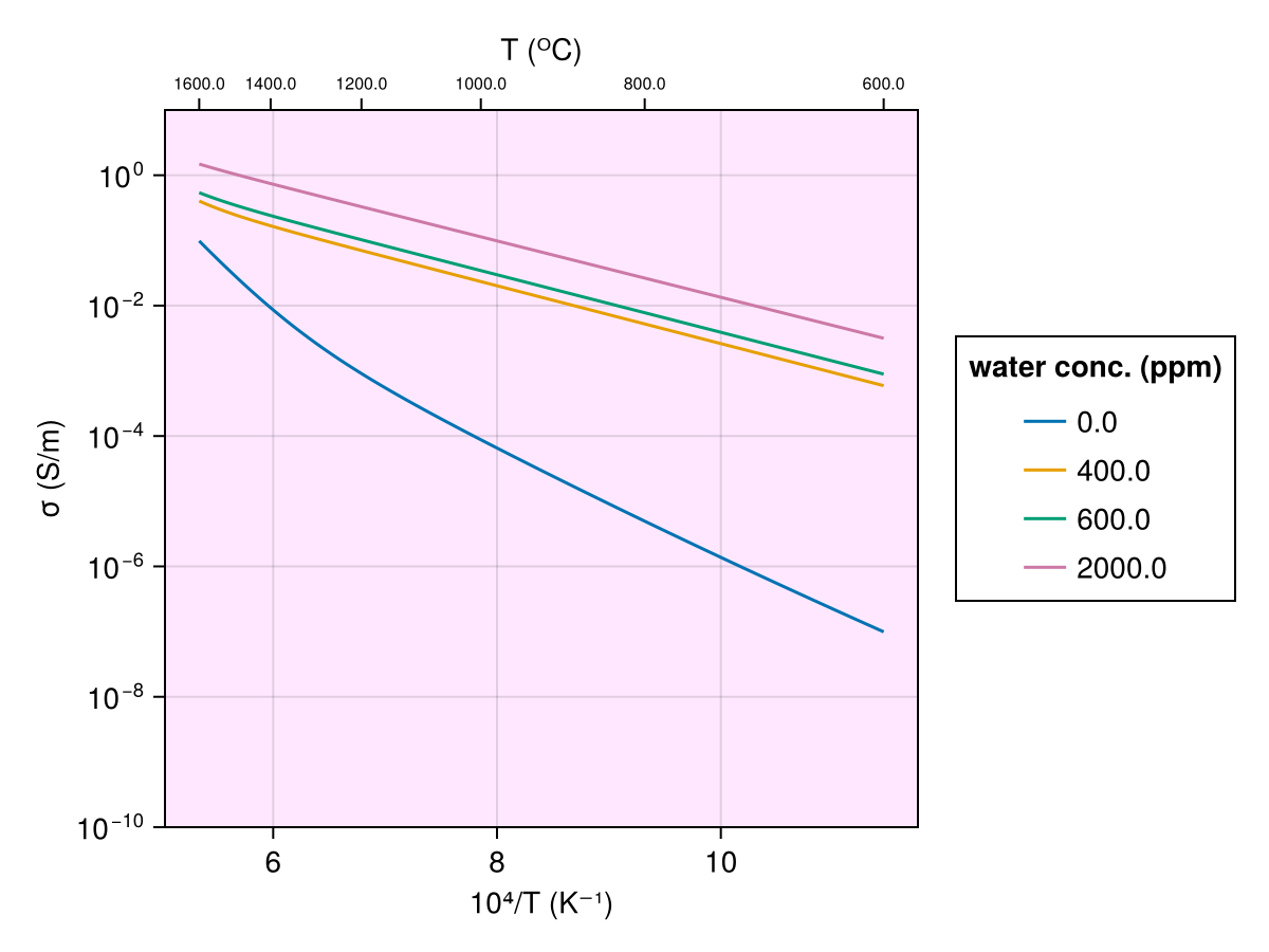

Melt

Ni2011

Porosity.Ni2011 Type

julia

Ni2011(T, Ch2o_m)

Electrical conductivity model for basaltic melt dependent on Temperature and water content in melt.

Arguments

T : Temperature of melt (should be greater than 1146.8 K)
Ch2o_m : water concentration in melt (in ppm)

Usage

julia

julia> model = Ni2011(1000 + 273.0, 2e4)
Model : Ni2011
Temperature (K) : 1273.0
Water concentration in melt (ppm) : 20000.0

julia> log_cond = forward(model, [])
Rock physics Response : RockphyCond
log₁₀ conductivity (S/m) : -2.3578741895190163

References

Ni, H., Keppler, H. & Behrens, H. (2011), "Electrical conductivity of hydrous basaltic melts: implications for partial melting in the upper mantle.", Contrib Mineral Petrol 162, 637–650 (2011), doi: https://doi.org/10.1007/s00410-011-0617-4

source

The distribution with temperature looks like :

Code for this figure

julia

f = Figure()
ax = Axis(f[1, 1]; yscale=log10, xlabel="10⁴/T (K⁻¹)", ylabel="σ (S/m)",
    yticks=LogTicks(WilkinsonTicks(9; k_min=8)), backgroundcolor=(:magenta, 0.05))

xts = inv.([1000, 1100, 1200, 1300, 1400] .+ 273.0) .* 1e4

ax2 = Axis(f[1, 1]; yscale=log10, xaxisposition=:top, yaxisposition=:right, xlabel="T (ᴼC)",
    xgridvisible=false, xtickformat=x -> string.(round.((1e4 ./ x) .- 273)),
    xticklabelsize=10, backgroundcolor=(:magenta, 0.05))
ax2.xticks = xts
hidespines!(ax2)
hideydecorations!(ax2)
linkyaxes!(ax, ax2)

T = (1000:1400) .+ 273.0
Ch2o = [0.0, 0.01, 0.03, 0.1]' .* 1e4
m = Ni2011(T, Ch2o)
logsig = forward(m, []).σ

for i in eachindex(Ch2o)
    w = Ch2o[i]
    lines!(ax, inv.(T) .* 1e4, 10 .^ logsig[:, i]; label="$w")
    lines!(ax2, inv.(T) .* 1e4, 10 .^ logsig[:, i]; alpha=0)
end

# ylims!(ax2, 1e-8, 1)
f[1, 2] = Legend(f, ax, "water conc. (ppm)")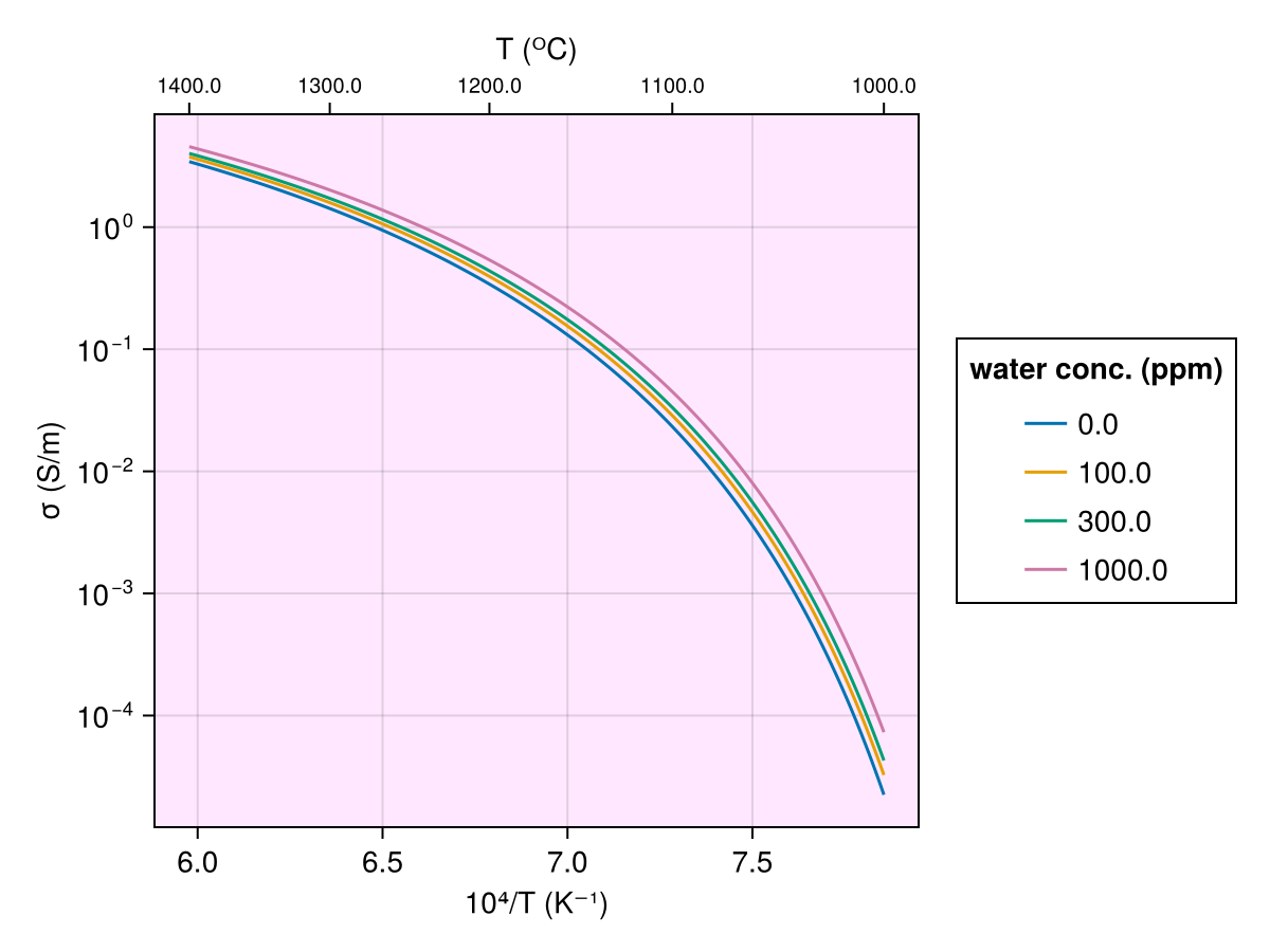

Sifre2014

Porosity.Ni2011 Type

julia

Ni2011(T, Ch2o_m)

Electrical conductivity model for basaltic melt dependent on Temperature and water content in melt.

Arguments

T : Temperature of melt (should be greater than 1146.8 K)
Ch2o_m : water concentration in melt (in ppm)

Usage

julia

julia> model = Ni2011(1000 + 273.0, 2e4)
Model : Ni2011
Temperature (K) : 1273.0
Water concentration in melt (ppm) : 20000.0

julia> log_cond = forward(model, [])
Rock physics Response : RockphyCond
log₁₀ conductivity (S/m) : -2.3578741895190163

References

Ni, H., Keppler, H. & Behrens, H. (2011), "Electrical conductivity of hydrous basaltic melts: implications for partial melting in the upper mantle.", Contrib Mineral Petrol 162, 637–650 (2011), doi: https://doi.org/10.1007/s00410-011-0617-4

source

The distribution with temperature looks like :

Code for this figure

julia

f = Figure()
ax = Axis(f[1, 1]; yscale=log10, xlabel="10⁴/T (K⁻¹)", ylabel="σ (S/m)",
    yticks=LogTicks(WilkinsonTicks(9; k_min=8)), backgroundcolor=(:magenta, 0.05))

xts = inv.([800, 1000, 1100, 1200, 1300, 1400] .+ 273.0) .* 1e4

ax2 = Axis(f[1, 1]; yscale=log10, xaxisposition=:top, yaxisposition=:right, xlabel="T (ᴼC)",
    xgridvisible=false, xtickformat=x -> string.(round.((1e4 ./ x) .- 273)),
    xticklabelsize=10, backgroundcolor=(:magenta, 0.05))
ax2.xticks = xts
hidespines!(ax2)
hideydecorations!(ax2)
linkyaxes!(ax, ax2)

T = (800:1400) .+ 273.0
Ch2o = [0.0, 0.01, 0.03, 0.1]' .* 1e4
Cco2_m = 1e3
m = Sifre2014(T, Ch2o, Cco2_m)
logsig = forward(m, []).σ

for i in eachindex(Ch2o)
    w = Ch2o[i]
    lines!(ax, inv.(T) .* 1e4, 10 .^ logsig[:, i]; label="$w")
    lines!(ax2, inv.(T) .* 1e4, 10 .^ logsig[:, i]; alpha=0)
end

f[1, 2] = Legend(f, ax, "water conc. (ppm)")

ax = Axis(f[2, 1]; yscale=log10, xlabel="10⁴/T (K⁻¹)", ylabel="σ (S/m)",
    yticks=LogTicks(WilkinsonTicks(9; k_min=8)), backgroundcolor=(:magenta, 0.05))

xts = inv.([800, 1000, 1100, 1200, 1300, 1400] .+ 273.0) .* 1e4

ax2 = Axis(f[2, 1]; yscale=log10, xaxisposition=:top, yaxisposition=:right, xlabel="T (ᴼC)",
    xgridvisible=false, xtickformat=x -> string.(round.((1e4 ./ x) .- 273)),
    xticklabelsize=10, backgroundcolor=(:magenta, 0.05))
ax2.xticks = xts
hidespines!(ax2)
hideydecorations!(ax2)
linkyaxes!(ax, ax2)

T = (1000:1400) .+ 273.0
Ch2o = 1e3
Cco2_m = [0.0, 0.01, 0.03, 0.1]' .* 1e4
m = Sifre2014(T, Ch2o, Cco2_m)
logsig = forward(m, []).σ

for i in eachindex(Cco2_m)
    w = Cco2_m[i]
    lines!(ax, inv.(T) .* 1e4, 10 .^ logsig[:, i]; label="$w")
    lines!(ax2, inv.(T) .* 1e4, 10 .^ logsig[:, i]; alpha=0)
end

f[2, 2] = Legend(f, ax, "CO₂ conc. (ppm)")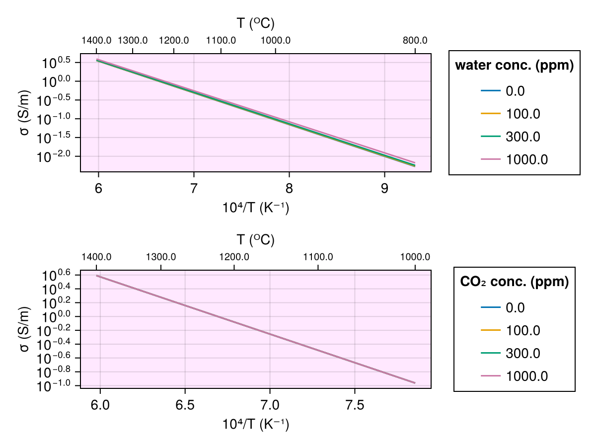

Gaillard2008

Porosity.Gaillard2008 Type

julia

Gaillard2008(T)

Electrical conductivity model for melt dependent on Temperature.

Usage

julia

julia> model = Gaillard2008(1000 + 273.0)
Model : Gaillard2008
Temperature (K) : 1273.0

julia> log_cond = forward(model, [])
Rock physics Response : RockphyCond
log₁₀ conductivity (S/m) : 2.2275677836002115

Arguments

T : Temperature of melt (should be greater than 1146.8 K)

References

Gaillard, Fabrice & Malki, Mohammed & Iacono-Marziano, Giada & Pichavant, Michel & Scaillet, Bruno. (2008), "Carbonatite Melts and Electrical Conductivity in the Asthenosphere", Science (New York, N.Y.). 322. 1363-5, doi: 10.1126/science.1164446.

source

The distribution with temperature looks like :

Code for this figure

julia

f = Figure()
ax = Axis(f[1, 1]; yscale=log10, xlabel="10⁴/T (K⁻¹)", ylabel="σ (S/m)",
    yticks=LogTicks(WilkinsonTicks(6; k_min=5)), backgroundcolor=(:magenta, 0.05))

xts = inv.([700, 900, 1100, 1300, 1500] .+ 273.0) .* 1e4

ax2 = Axis(f[1, 1]; yscale=log10, xaxisposition=:top, yaxisposition=:right, xlabel="T (ᴼC)",
    xgridvisible=false, xtickformat=x -> string.(round.((1e4 ./ x) .- 273)),
    xticklabelsize=10, backgroundcolor=(:magenta, 0.05))
ax2.xticks = xts
hidespines!(ax2)
hideydecorations!(ax2)
linkyaxes!(ax, ax2)

T = (700:1600) .+ 273.0
m = Gaillard2008(T)
logsig = forward(m, []).σ

lines!(ax, inv.(T) .* 1e4, 10 .^ logsig)
lines!(ax2, inv.(T) .* 1e4, 10 .^ logsig; alpha=0)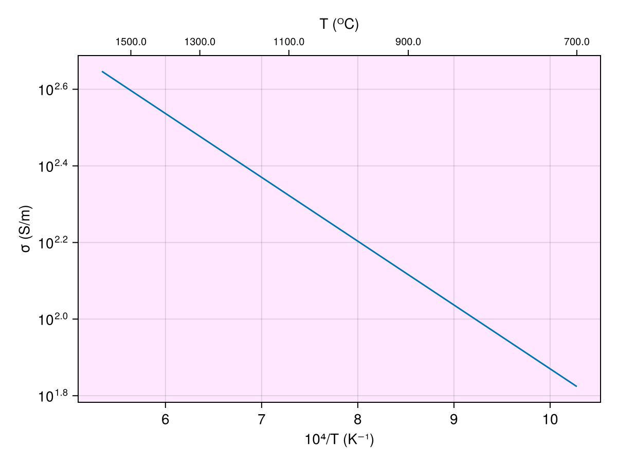

Orthopyroxene

Dai_Karato2009

Porosity.Dai_Karato2009 Type

julia

Dai_Karato2009(T, Ch2o_opx)

Electrical conductivity model for olivine dependent on temperature and water concentration.

Arguments

T : Temperature of olivine (in K)
Ch2o_opx : water concentration in orthopyroxene (in ppm)

References

Dai, Lidong and Karato, Shun-ichiro (2009), "Electrical conductivity of orthopyroxene: Implications for the water content of the asthenosphere", Proceedings of the Japan Academy, Series B, doi:10.2183/pjab.85.466

Usage

julia

julia> model = Dai_Karato2009(1000 + 273.0, 2e4)
Model : Dai_Karato2009
Temperature (K) : 1273.0
Water concentration in orthopyroxene (ppm) : 20000.0

julia> log_cond = forward(model, [])
Rock physics Response : RockphyCond
log₁₀ conductivity (S/m) : -1.4966847149880984

source

The distribution with temperature looks like :

Code for this figure

julia

f = Figure()

ax = Axis(f[1, 1]; yscale=log10, xlabel="10⁴/T (K⁻¹)", ylabel="σ (S/m)",
    yticks=LogTicks(WilkinsonTicks(6; k_min=5)), backgroundcolor=(:magenta, 0.05))

xts = inv.([800, 900, 1000, 1300] .+ 273.0) .* 1e4

ax2 = Axis(f[1, 1]; yscale=log10, xaxisposition=:top, yaxisposition=:right, xlabel="T (ᴼC)",
    xgridvisible=false, xtickformat=x -> string.(round.((1e4 ./ x) .- 273)),
    xticklabelsize=8, backgroundcolor=(:magenta, 0.05))
ax2.xticks = xts
hidespines!(ax2)
hideydecorations!(ax2)
linkyaxes!(ax, ax2)

T = (700:1300) .+ 273.0
Ch2o = [0.0, 100, 200, 2000]'
m = Dai_Karato2009(T, Ch2o)
logsig = forward(m, []).σ

for i in eachindex(Ch2o)
    w = Ch2o[i]
    lines!(ax, inv.(T) .* 1e4, 10 .^ logsig[:, i]; label="$w")
    lines!(ax2, inv.(T) .* 1e4, 10 .^ logsig[:, i]; alpha=0)
end
f[1, 2] = Legend(f, ax, "water conc. (ppm)")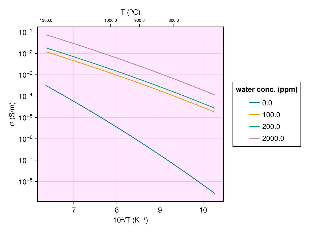

Zhang2012

Porosity.Zhang2012 Type

julia

Zhang2012(T, Ch2o_opx)

Electrical conductivity model for olivine dependent on temperature and water concentration.

Arguments

T : Temperature of olivine (in K)
Ch2o_opx : water concentration in olivine (in ppm)

References

todo

Usage

julia

julia> model = Zhang2012(1000 + 273.0, 2e4)
Model : Zhang2012
Temperature (K) : 1273.0
Water concentration in orthopyroxene (ppm) : 20000.0

julia> log_cond = forward(model, [])
Rock physics Response : RockphyCond
log₁₀ conductivity (S/m) : -0.045414286402875675

source

The distribution with temperature looks like (compare with fig. 6 in Zhang et al., 2012):

Code for this figure

julia

f = Figure()

ax = Axis(f[1, 1]; yscale=log10, xlabel="10⁴/T (K⁻¹)", ylabel="σ (S/m)",
    yticks=LogTicks(WilkinsonTicks(6; k_min=5)), backgroundcolor=(:magenta, 0.05))

xts = inv.([800, 1300.0, 2000.0] .+ 273.0) .* 1e4

ax2 = Axis(f[1, 1]; yscale=log10, xaxisposition=:top, yaxisposition=:right, xlabel="T (ᴼC)",
    xgridvisible=false, xtickformat=x -> string.(round.((1e4 ./ x) .- 273)),
    xticklabelsize=8, backgroundcolor=(:magenta, 0.05))
ax2.xticks = xts
hidespines!(ax2)
hideydecorations!(ax2)
linkyaxes!(ax, ax2)

T = (700:2600) .+ 273.0
Ch2o = [0.0, 1, 10, 100, 1000, 10000]'
m = Zhang2012(T, Ch2o)
logsig = forward(m, []).σ

for i in eachindex(Ch2o)
    w = Ch2o[i]
    lines!(ax, inv.(T) .* 1e4, 10 .^ logsig[:, i]; label="$w")
    lines!(ax2, inv.(T) .* 1e4, 10 .^ logsig[:, i]; alpha=0)
end

f[1, 2] = Legend(f, ax, "water conc. (ppm)")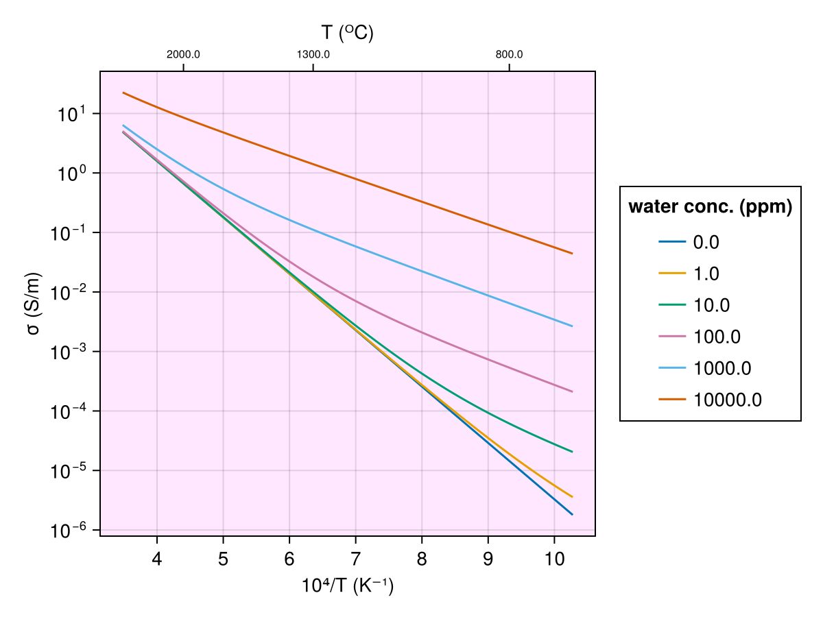

Clinopyroxene

Yang2011

Porosity.Yang2011 Type

julia

Yang2011(T, Ch2o_cpx)

Electrical conductivity model for olivine dependent on temperature and water concentration.

Arguments

T : Temperature of olivine (in K)
Ch2o_cpx : water concentration in olivine (in ppm)

References

Yang, Xiaozhi and Keppler, Hans and McCammon, Catherine and Ni, Huaiwei and Xia, Qunke and Fan, Qicheng (2011), "Effect of water on the electrical conductivity of lower crustal clinopyroxene", Journal of Geophysical Research, doi:https://doi.org/10.1029/2010JB008010

Usage

julia

julia> model = Yang2011(1000 + 273.0, 2e4)
Model : Yang2011
Temperature (K) : 1273.0
Water concentration in clinopyroxene (ppm) : 20000.0

julia> log_cond = forward(model, [])
Rock physics Response : RockphyCond
log₁₀ conductivity (S/m) : 1.0103884511392625

source

The distribution with temperature looks like (compare with fig. 8 in Yang et al., 2011):

Code for this figure

julia

f = Figure()

ax = Axis(f[1, 1]; yscale=log10, xlabel="10⁴/T (K⁻¹)", ylabel="σ (S/m)",
    yticks=LogTicks(WilkinsonTicks(6; k_min=5)), backgroundcolor=(:magenta, 0.05))

xts = inv.([400, 500, 800, 1000, 1300] .+ 273.0) .* 1e4

ax2 = Axis(f[1, 1]; yscale=log10, xaxisposition=:top, yaxisposition=:right, xlabel="T (ᴼC)",
    xgridvisible=false, xtickformat=x -> string.(round.((1e4 ./ x) .- 273)),
    xticklabelsize=8, backgroundcolor=(:magenta, 0.05))
ax2.xticks = xts
hidespines!(ax2)
hideydecorations!(ax2)
linkyaxes!(ax, ax2)

T = (400:1300) .+ 273.0
Ch2o = [0.0, 100, 200, 2000]'
m = Yang2011(T, Ch2o)
logsig = forward(m, []).σ

for i in eachindex(Ch2o)
    w = Ch2o[i]
    lines!(ax, inv.(T) .* 1e4, 10 .^ logsig[:, i]; label="$w")
    lines!(ax2, inv.(T) .* 1e4, 10 .^ logsig[:, i]; alpha=0)
end
f[1, 2] = Legend(f, ax, "water conc. (ppm)")

Conductivity models ​

Minerals ​

SEO3 ​

Wang2006 ​

Yoshino2009 ​

Poe2010 ​

Jones2012 ​

UHO2014 ​

Melt ​

Ni2011 ​

Sifre2014 ​

Gaillard2008 ​

Orthopyroxene ​

Dai_Karato2009 ​

Zhang2012 ​

Clinopyroxene ​

Yang2011 ​

Conductivity models

Minerals

SEO3

Wang2006

Yoshino2009

Poe2010

Jones2012

UHO2014

Melt

Ni2011

Sifre2014

Gaillard2008

Orthopyroxene

Dai_Karato2009

Zhang2012

Clinopyroxene

Yang2011