Anelastic models
Andrade pseudoperiod model
Porosity.andrade_psp Type
andrade_psp(T, P, dg, σ, ϕ, ρ, f)Calculate anelastic properties stored in RockPhyAnelastic using the Andrade model with pseudo-scaling per Jackson and Faul (2010)
Arguments
- `T` : Temperature of the rock (K)
- `P` : Pressure (GPa)
- `dg`: Grain size (μm)
- `σ` : Shear stress (GPa)
- `ϕ` : Porosity
- `ρ` : Density (kg/m³)
- `f` : frequency
Keyword Arguments
- `params` : Various coefficients required for calculation.
Also holds coefficients and the type of `RockphyElastic` model to be used.

To investigate coefficients, call `default_params(Val{andrade_psp}())`.
To modify coefficients, check the relevant documentation page. This
will also users to pick any particular type of `RockphyElastic` model, defaults to `anharmonic`.
Usage
Note
Make sure that the dimension of vector f is one more than the other parameters. Check relevant tutorials. Note the transpose on f when making the model in the following eg.
julia> T = [800, 1000] .+ 273.0f0;

julia> P = 2 .+ zero(T);

julia> dg = 4.0f0;

julia> σ = 10.0f-3;

julia> ϕ = 1.0f-2;

julia> ρ = 3300.0f0;

julia> f = [1.0f0, 1.0f1];

julia> model = andrade_psp(T, P, dg, σ, ϕ, ρ, f')
Model : andrade_psp
Temperature (K) : Float32[1073.0, 1273.0]
Pressure (GPa) : Float32[2.0, 2.0]
grain size(μm) : 4.0
Shear stress (GPa) : 0.01
Porosity : 0.01
Density (kg/m³) : 3300.0
Frequency (Hz) : Float32[1.0 10.0]

julia> forward(model, [])
Rock physics Response : RockphyAnelastic
Real part of dynamic compliance (Pa⁻¹) : Float32[1.35194625f-11 1.35077696f-11; 1.4162938f-11 1.4082101f-11]
Imaginary part of dynamic compliance (Pa⁻¹) : Float32[1.259776f-14 5.8473344f-15; 8.712478f-14 4.0431112f-14]
Attenuation : Float32[0.00093182403 0.00043288674; 0.006151603 0.0028710994]
Modulus (Pa) : Float32[7.39674f10 7.403146f10; 7.060549f10 7.1011836f10]
Anelastic S-wave velocity : (m/s) : Float32[4734.381 4736.4307; 4625.538 4638.8296]
Frequency averaged S-wave velocity (m/s) : Float32[4735.406, 4632.1836]
References
- Jackson and Faul, 2010, "Grainsize-sensitive viscoelastic relaxation in olivine: Towards a robust laboratory-based model for seismological application", Phys. Earth Planet. Inter., https://doi.org/10.1016/j.pepi.2010.09.005
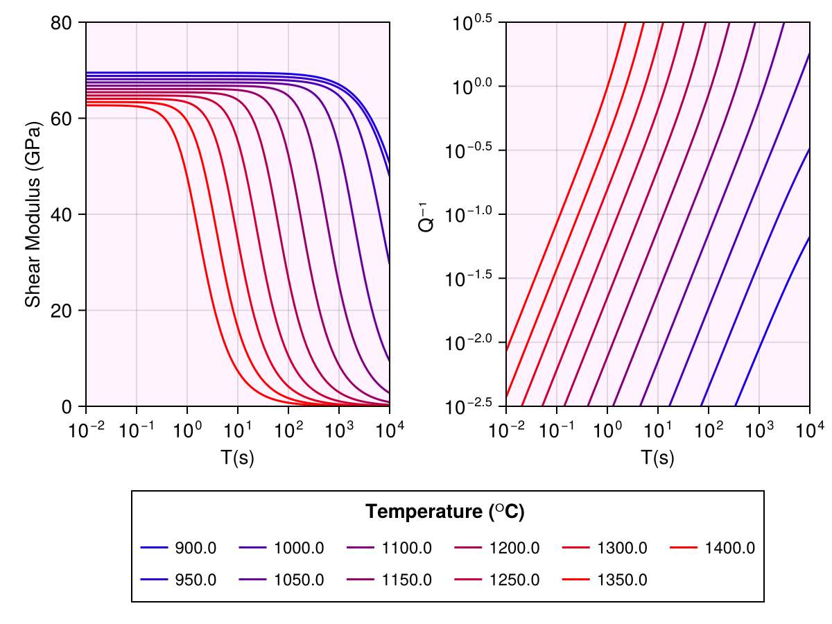
For different temperatures, the distribution with oscillation period looks like (compare with Fig. 1 (e) and (f) of Jackson and Faul, 2010)
Tip
The following code is a nice beginner example on changing params values for rock physics models
Code for this figure
T = (900:50:1200) .+ 273.0
P = 0.2
dg = 3.1
σ = 10.0 * 1.0f-3
ϕ = 0.0
ρ = 3300.0

f = 10 .^ -collect(range(0, 3; length=100))

params = default_params(andrade_psp)
params_elastic = default_params(anharmonic)
@unpack T_K_ref, dG_dT, dG_dP, P_Pa_ref = params_elastic
new_Gu_ol = 1e-9 * (params.G_UR * 1e9 - (900 + 273 - T_K_ref) * dG_dT -
             (0.2 * 1e9 - P_Pa_ref) * dG_dP)

new_params_elastic = (; params_elastic..., Gu_0_ol=new_Gu_ol)

new_params = (; params..., params_elastic=new_params_elastic)

m = andrade_psp(T, P, dg, σ, ϕ, ρ, f')

resp = forward(m, [], new_params);
size(resp.J1)

fig = Figure()
ax = Axis(fig[1, 1]; xscale=log10, backgroundcolor=(:magenta, 0.05),
    ylabel="Shear Modulus (GPa)", xlabel="T(s)")

for i in eachindex(T)
    color_ = RGBf(i / 10, 0.0, 1 - i / 10)
    lines!(ax, 1 ./ f, resp.M[i, :] ./ (1e9); color=color_, label="$(T[i] - 273)")
end
xlims!(ax, 1e-2, 1e4)
ylims!(ax, 0, 80)

ax2 = Axis(fig[1, 2]; xscale=log10, yscale=log10,
    backgroundcolor=(:magenta, 0.05), ylabel="Q⁻¹ ", xlabel="T(s)")

for i in eachindex(T)
    color_ = RGBf(i / 10, 0.0, 1 - i / 10)
    lines!(ax2, 1 ./ f, resp.Qinv[i, :]; color=color_, label="$(T[i] - 273)")
end
xlims!(ax2, 1e-2, 1e4)
ylims!(ax2, 10.0^(-2.5), 10.0^0.5)
fig[2, 1:2] = Legend(fig, ax, "Temperature"; orientation=:horizontal, labelsize=12)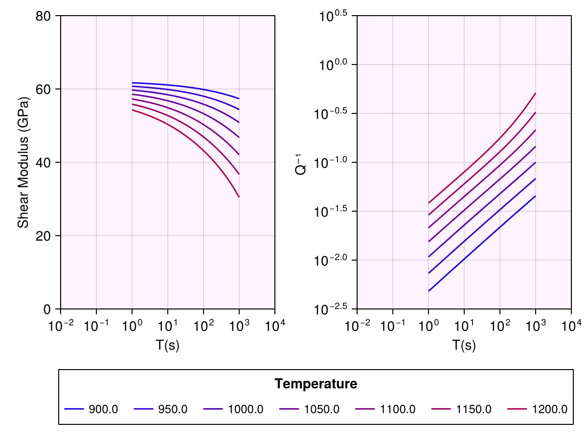
Extended Burgers model
Porosity.eburgers_psp Type
eburgers_psp(T, P, dg, σ, ϕ, ρ, Ch2o_ol, T_solidus, f)Calculate anelastic properties stored in RockphyAnelastic using the Extended Burgers model with pseudo-scaling per Jackson and Faul (2010)
Arguments
- `T` : Temperature of the rock (K)
- `P` : Pressure (GPa)
- `dg`: Grain size (μm)
- `σ` : Shear stress (GPa)
- `ϕ` : Porosity
- `ρ` : Density (kg/m³)
- `Ch2o_ol` : water concentration in olivine (in ppm)
- `T_solidus` : Solidus temperature (K), only used when using `xfit_premelt` for viscosity calculations, when scaling from Jackson and Faul (2010) for maxwell time calculations is not used
- `f` : frequency
Keyword Arguments
- `params` : Various coefficients required for calculation.
Also holds coefficients and the type of `RockphyElastic` model and `RockphyViscous model` to be used.

To investigate coefficients, call `default_params(Val{eburgers_psp}())`.
To modify coefficients, check the relevant documentation page. This
will also users to pick any particular type of `RockphyElastic` model, defaults to `anharmonic`,
as well as `RockphyViscous` model (for diffusion-derived viscosity), defaults to `xfit_premelt`

`params` for `eburgers_psp` holds a few important fields:
    - `params_btype` : fitting parameters from Jackson and Faul (2010) to be used, defaults to `bg_only`.
    Available options are :
        - `bg_only` : multiple sample best high-temp background only fit
        - `bg_peak` : multiple sample best high-temp background + peak fit
        - `s6585_bg_only` : single sample 6585 fit, HTB only
        - `s6585_bg_peak` : single sample 6585 fit, HTB + dissipation peak

    - `melt_enhancement` : TODO

    -  `JF10_visc` : Whether to use scaling from Jackson and Faul (2010) for maxwell time calculations,
    otherwise calculate them using the `RockphyViscous` model provide. **Defaults to `true`.**

    - `integration_params` : Tells which integration option to be used,
    and the number of points (Should not be touched ideally!)
    Available options are `quadgk`, `trapezoidal` and `simpson`, defaults to `quadgk`.
Usage
Note
Make sure that the dimension of vector f is one more than the other parameters. Check relevant tutorials. Note the transpose on f when making the model in the following eg.
julia> T = [800, 1000] .+ 273.0f0;

julia> P = 2 .+ zero(T);

julia> dg = 4.0f0;

julia> σ = 10.0f-3;

julia> ϕ = 1.0f-2;

julia> ρ = 3300.0f0;

julia> Ch2o_ol = 0.0f0;

julia> T_solidus = 900 + 273.0f0;

julia> f = [1.0f0, 1.0f1];

julia> model = eburgers_psp(T, P, dg, σ, ϕ, ρ, Ch2o_ol, T_solidus, f')
Model : eburgers_psp
Temperature (K) : Float32[1073.0, 1273.0]
Pressure (GPa) : Float32[2.0, 2.0]
grain size(μm) : 4.0
Shear stress (GPa) : 0.01
Porosity : 0.01
Density (kg/m³) : 3300.0
Water concentration in olivine (ppm) : 0.0
Solidus Temperature (K) : 1173.0
Frequency (Hz) : Float32[1.0 10.0]

julia> forward(model, [])
Rock physics Response : RockphyAnelastic
Real part of dynamic compliance (Pa⁻¹) : Float32[1.3524236f-11 1.3499646f-11; 1.42722735f-11 1.413697f-11]
Imaginary part of dynamic compliance (Pa⁻¹) : Float32[2.754988f-14 8.080778f-15; 1.29419f-13 7.1557296f-14]
Attenuation : Float32[0.0020370746 0.00059859187; 0.009067862 0.0050617135]
Modulus (Pa) : Float32[7.394117f10 7.4076004f10; 7.006304f10 7.073561f10]
Anelastic S-wave velocity : (m/s) : Float32[4733.5415 4737.8555; 4607.7354 4629.7983]
Frequency averaged S-wave velocity (m/s) : Float32[4735.698, 4618.7666]
References
Faul and Jackson, 2015, "Transient Creep and Strain Energy Dissipation: An Experimental Perspective", Ann. Rev. of Earth and Planetary Sci., https://doi.org/10.1146/annurev-earth-060313-054732
Jackson and Faul, 2010, "Grainsize-sensitive viscoelastic relaxation in olivine: Towards a robust laboratory-based model for seismological application", Phys. Earth Planet. Inter., https://doi.org/10.1016/j.pepi.2010.09.005
For different temperatures, the distribution with oscillation period looks like (compare with Fig. 1 (a) and (b) of Jackson and Faul, 2010)
Code for this figure
T = (600:50:1200) .+ 273.0
P = 0.2
dg = 3.1
σ = 10.0 * 1.0f-3
ϕ = 0.0
ρ = 3300.0

f = 10 .^ -collect(range(-2, 4; length=100))

m = eburgers_psp(T, P, dg, σ, ϕ, ρ, f')
resp = forward(m, []);
size(resp.J1)

fig = Figure()
ax = Axis(fig[1, 1]; xscale=log10, backgroundcolor=(:magenta, 0.05),
    ylabel="Shear Modulus (GPa)", xlabel="T(s)")

for i in eachindex(T)
    color_ = RGBf(i / 10, 0.0, 1 - i / 10)
    lines!(ax, 1 ./ f, resp.M[i, :] ./ (1e9); color=color_, label="$(T[i] - 273)")
end
xlims!(ax, 1e-2, 1e4)
ylims!(ax, 0, 80)

ax2 = Axis(fig[1, 2]; xscale=log10, yscale=log10,
    backgroundcolor=(:magenta, 0.05), ylabel="Q⁻¹ ", xlabel="T(s)")

for i in eachindex(T)
    color_ = RGBf(i / 10, 0.0, 1 - i / 10)
    lines!(ax2, 1 ./ f, resp.Qinv[i, :]; color=color_, label="$(T[i] - 273)")
end
xlims!(ax2, 1e-2, 1e4)
ylims!(ax2, 10.0^(-2.5), 10.0^0.5)
fig[2, 1:2] = Legend(
    fig, ax, "Temperature"; orientation=:horizontal, labelsize=12, nbanks=2)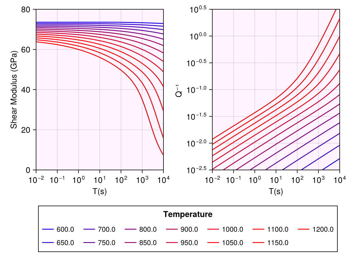
Warn
Use of peak coefficients is highly discouraged because these involve integrals that can be unstable in their limits. Note that the figures are skewed and the weird behaviour increases at lower temperatures.
Similar figures for different params can be obtained (compare with Fig. 1 (c) and (d) of Jackson and Faul, 2010):
Tip
The following code is a nice example on changing params values for rock physics models
Code for this figure
T = (600:50:1200) .+ 273.0
P = 0.2
dg = 3.1
σ = 10.0 * 1.0f-3
ϕ = 0.0
ρ = 3300.0

params = default_params(eburgers_psp)
params_elastic = default_params(anharmonic)
@unpack T_K_ref, dG_dT, dG_dP, P_Pa_ref = params_elastic
new_Gu_ol = 1e-9 *
            (Porosity.params_JF10.s6585_bg_peak.G_UR * 1e9 - (900 + 273 - T_K_ref) * dG_dT -
             (0.2 * 1e9 - P_Pa_ref) * dG_dP)

new_params_elastic = (; params_elastic..., Gu_0_ol=new_Gu_ol)

new_params = (; params..., params_elastic=new_params_elastic,
    params_btype=Porosity.params_JF10.s6585_bg_peak)

m = eburgers_psp(T, P, dg, σ, ϕ, ρ, f')

resp = forward(m, [], new_params);
size(resp.J1)

fig = Figure(; size=(700, 400))
ax = Axis(fig[1, 1]; xscale=log10, backgroundcolor=(:magenta, 0.05),
    ylabel="Shear Modulus (GPa)", xlabel="T(s)")

for i in eachindex(T)
    color_ = RGBf(i / 10, 0.0, 1 - i / 10)
    lines!(ax, 1 ./ f, resp.M[i, :] ./ (1e9); color=color_, label="$(T[i] - 273)")
end
xlims!(ax, 1e-2, 1e4)
ylims!(ax, 0, 80)

ax2 = Axis(fig[1, 2]; xscale=log10, yscale=log10,
    backgroundcolor=(:magenta, 0.05), ylabel="Q⁻¹ ", xlabel="T(s)")

for i in eachindex(T)
    color_ = RGBf(i / 10, 0.0, 1 - i / 10)
    lines!(ax2, 1 ./ f, resp.Qinv[i, :]; color=color_, label="$(T[i] - 273)")
end
xlims!(ax2, 1e-2, 1e4)
ylims!(ax2, 10.0^(-2.5), 10.0^0.5)
fig[2, 1:2] = Legend(
    fig, ax, "Temperature"; orientation=:horizontal, labelsize=12, nbanks=2)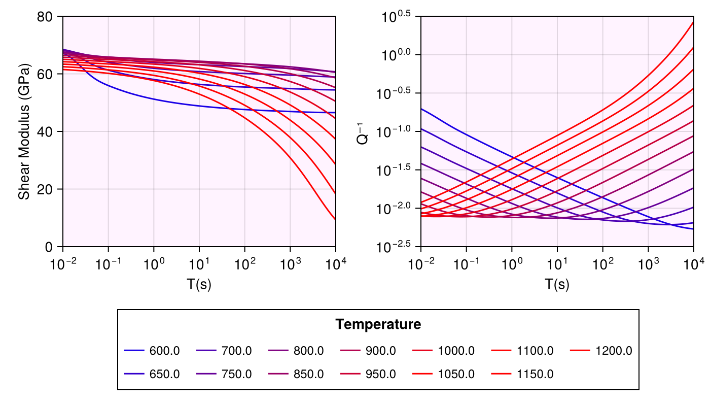
Premelt model
Porosity.premelt_anelastic Type
premelt_anelastic(T, P, dg, σ, ϕ, ρ, T_solidus, Ch2o_ol, f)Calculate anelastic properties stored in RockPhyAnelastic using the Master curve maxwell scaling per near-solidus parametrization of Yamauchi and Takei (2016), with optional extension to include direct melt effects of Yamauchi and Takei (2024)
Arguments
- `T` : Temperature of the rock (K)
- `P` : Pressure (GPa)
- `dg`: Grain size (μm)
- `σ` : Shear stress (GPa)
- `ϕ` : Porosity
- `ρ` : Density (kg/m³)
- `Ch2o_ol` : water concentration in olivine (in ppm)
- `T_solidus` : Solidus temperature (K)
- `f` : frequency
Keyword Arguments
- `params` : Various coefficients required for calculation.
Also holds coefficients and the type of `RockphyElastic` model and `RockphyViscous model` to be used.

To investigate coefficients, call `default_params(Val{xfit_premelt}())`.
To modify coefficients, check the relevant documentation page. This
will also users to pick any particular type of `RockphyElastic` model, defaults to `anharmonic`.

`params` for `premelt_anelastic` holds another important field:
    - `include_direct_melt_effect` : Whether to include the melt effect of Yamauchi and Takei (2024), defaults to false
Usage
Note
Make sure that the dimension of vector f is one more than the other parameters. Check relevant tutorials. Note the transpose on f when making the model in the following eg.
julia> T = [800, 1000] .+ 273.0f0;

julia> P = 2 .+ zero(T);

julia> dg = 4.0f0;

julia> σ = 10.0f-3;

julia> ϕ = 1.0f-2;

julia> ρ = 3300.0f0;

julia> Ch2o_ol = 0.0f0;

julia> T_solidus = 900 + 273.0f0;

julia> f = [1.0f0, 1.0f1];

julia> model = premelt_anelastic(T, P, dg, σ, ϕ, ρ, Ch2o_ol, T_solidus, f')
Model : premelt_anelastic
Temperature (K) : Float32[1073.0, 1273.0]
Pressure (GPa) : Float32[2.0, 2.0]
grain size(μm) : 4.0
Shear stress (GPa) : 0.01
Porosity : 0.01
Density (kg/m³) : 3300.0
Water concentration in olivine (ppm) : 0.0
Solidus Temperature (K) : 1173.0
Frequency (Hz) : Float32[1.0 10.0]

julia> forward(model, [])
Rock physics Response : RockphyAnelastic
Real part of dynamic compliance (Pa⁻¹) : Float32[1.3508699f-11 1.3501298f-11; 1.7620908f-11 1.6476176f-11]
Imaginary part of dynamic compliance (Pa⁻¹) : Float32[8.801486f-15 2.5916762f-15; 8.878848f-13 6.8378257f-13]
Attenuation : Float32[0.0006515421 0.00019195756; 0.050388142 0.041501287]
Modulus (Pa) : Float32[7.402635f10 7.406695f10; 5.6678855f10 6.0641493f10]
Anelastic S-wave velocity : (m/s) : Float32[4736.267 4737.566; 4144.3228 4286.748]
Frequency averaged S-wave velocity (m/s) : Float32[4736.9165, 4215.535]
References
Yamauchi and Takei, 2016, "Polycrystal anelasticity at near-solidus temperatures", J. Geophys. Res. Solid Earth, https://doi.org/10.1002/2016JB013316
Yamauchi and Takei, 2024, "Effect of Melt on Polycrystal Anelasticity", J. Geophys. Res. Solid Earth, https://doi.org/10.1029/2023JB027738
For different temperatures, the distribution with oscillation period looks like
Code for this figure
T = (600:50:1400) .+ 273.0
P = 0.2
dg = 3.1
σ = 10.0 * 1.0f-3
ϕ = 0.0
ρ = 3300.0
T_solidus = 1100 + 273.0

f = 10 .^ -collect(range(-2, 4; length=100))

m = premelt_anelastic(T, P, dg, σ, ϕ, ρ, 0.0, T_solidus, f')

resp = forward(m, []);
size(resp.J1)

fig = Figure()
ax = Axis(fig[1, 1]; xscale=log10, backgroundcolor=(:magenta, 0.05),
    ylabel="Shear Modulus (GPa)", xlabel="T(s)")

for i in eachindex(T)
    color_ = RGBf(i / 10, 0.0, 1 - i / 10)
    lines!(ax, 1 ./ f, resp.M[i, :] ./ (1e9); color=color_, label="$(T[i] - 273)")
end
xlims!(ax, 1e-2, 1e4)
ylims!(ax, 0, 80)

ax2 = Axis(fig[1, 2]; xscale=log10, yscale=log10,
    backgroundcolor=(:magenta, 0.05), ylabel="Q⁻¹ ", xlabel="T(s)")

for i in eachindex(T)
    color_ = RGBf(i / 10, 0.0, 1 - i / 10)
    lines!(ax2, 1 ./ f, resp.Qinv[i, :]; color=color_, label="$(T[i] - 273)")
end
xlims!(ax2, 1e-2, 1e4)
ylims!(ax2, 10.0^(-2.5), 10.0^0.5)
fig[2, 1:2] = Legend(
    fig, ax, "Temperature (ᴼC) "; orientation=:horizontal, labelsize=12, nbanks=3)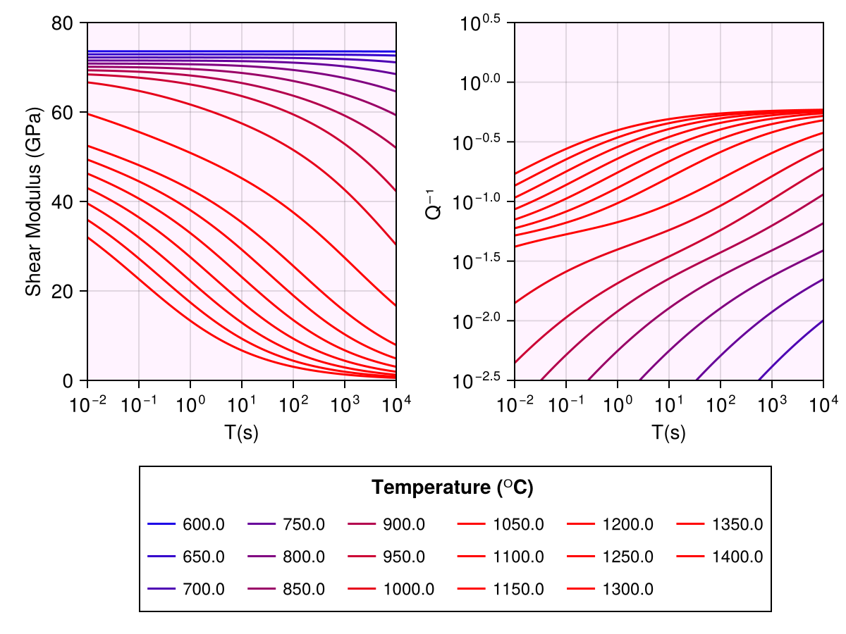
Master curve maxwell scaling model
Porosity.xfit_mxw Type
xfit_mxw(T, P, dg, σ, ϕ, ρ, T_solidus, Ch2o_ol, f)Calculate anelastic properties stored in RockPhyAnelastic using the Master curve maxwell scaling per McCarthy, Takei and Hiraga (2011)
Arguments
- `T` : Temperature of the rock (K)
- `P` : Pressure (GPa)
- `dg`: Grain size (μm)
- `σ` : Shear stress (GPa)
- `ϕ` : Porosity
- `ρ` : Density (kg/m³)
- `Ch2o_ol` : water concentration in olivine (in ppm)
- `T_solidus` : Solidus temperature (K), only used when using `xfit_premelt` for viscosity calculations
- `f` : frequency
Keyword Arguments
- `params` : Various coefficients required for calculation.
Available options are `fit1` and `fit2`, defaults to `fit1`, i.e, `params_xfit_mxw.fit1`
Also holds coefficients and the type of `RockphyElastic` model and `RockphyViscous model` to be used.

To investigate coefficients, call `default_params(Val{xfit_premelt}())`.
To modify coefficients, check the relevant documentation page. This
will also users to pick any particular type of `RockphyElastic` model, defaults to `anharmonic`,
as well as `RockphyViscous` model (for diffusion-derived viscosity), defaults to `xfit_mxw`
Usage
Note
Make sure that the dimension of vector f is one more than the other parameters. Check relevant tutorials. Note the transpose on f when making the model in the following eg.
julia> T = [800, 1000] .+ 273.0f0;

julia> P = 2 .+ zero(T);

julia> dg = 4.0f0;

julia> σ = 10.0f-3;

julia> ϕ = 1.0f-2;

julia> ρ = 3300.0f0;

julia> Ch2o_ol = 0.0f0;

julia> T_solidus = 900 + 273.0f0;

julia> f = [1.0f0, 1.0f1];

julia> model = xfit_mxw(T, P, dg, σ, ϕ, ρ, Ch2o_ol, T_solidus, f')
Model : xfit_mxw
Temperature (K) : Float32[1073.0, 1273.0]
Pressure (GPa) : Float32[2.0, 2.0]
grain size(μm) : 4.0
Shear stress (GPa) : 0.01
Porosity : 0.01
Density (kg/m³) : 3300.0
Water concentration in olivine (ppm) : 0.0
Solidus Temperature (K) : 1173.0
Frequency (Hz) : Float32[1.0 10.0]

julia> forward(model, [])
Rock physics Response : RockphyAnelastic
Real part of dynamic compliance (Pa⁻¹) : Float32[1.4031399f-11 1.3812445f-11; 1.6433199f-11 1.57985f-11]
Imaginary part of dynamic compliance (Pa⁻¹) : Float32[1.6107535f-13 1.3877004f-13; 5.1549807f-13 3.6455504f-13]
Attenuation : Float32[0.011479636 0.01004674; 0.031369306 0.023075296]
Modulus (Pa) : Float32[7.1264035f10 7.2394826f10; 6.0822508f10 6.3280304f10]
Anelastic S-wave velocity : (m/s) : Float32[4647.0596 4683.783; 4293.141 4379.024]
Frequency averaged S-wave velocity (m/s) : Float32[4665.4214, 4336.0825]
References
- McCarthy, Takei, Hiraga, 2011, "Experimental study of attenuation and dispersion over a broad frequency range:
- The universal scaling of polycrystalline materials", Journal of Geophy Research, http://dx.doi.org/10.1029/2011JB008384
For different temperatures, the distribution with oscillation period looks like
Code for this figure
T = (900:50:1400) .+ 273.0
P = 0.2
dg = 3.1
σ = 10.0 * 1.0f-3
ϕ = 0.0
ρ = 3300.0
Ch2o_ol = 0.0
T_solidus = 1100 + 273.0

f = 10 .^ -collect(range(-2, 4; length=100))

m = xfit_mxw(T, P, dg, σ, ϕ, ρ, Ch2o_ol, T_solidus, f')

resp = forward(m, []);
size(resp.J1)

fig = Figure()
ax = Axis(fig[1, 1]; xscale=log10, backgroundcolor=(:magenta, 0.05),
    ylabel="Shear Modulus (GPa)", xlabel="T(s)")

for i in eachindex(T)
    color_ = RGBf(i / 10, 0.0, 1 - i / 10)
    lines!(ax, 1 ./ f, resp.M[i, :] ./ (1e9); color=color_, label="$(T[i] - 273)")
end
xlims!(ax, 1e-2, 1e4)
ylims!(ax, 0, 80)

ax2 = Axis(fig[1, 2]; xscale=log10, yscale=log10,
    backgroundcolor=(:magenta, 0.05), ylabel="Q⁻¹ ", xlabel="T(s)")

for i in eachindex(T)
    color_ = RGBf(i / 10, 0.0, 1 - i / 10)
    lines!(ax2, 1 ./ f, resp.Qinv[i, :]; color=color_, label="$(T[i] - 273)")
end
xlims!(ax2, 1e-2, 1e4)
ylims!(ax2, 10.0^(-2.5), 10.0^0.5)
fig[2, 1:2] = Legend(
    fig, ax, "Temperature (ᴼC) "; orientation=:horizontal, labelsize=12, nbanks=2)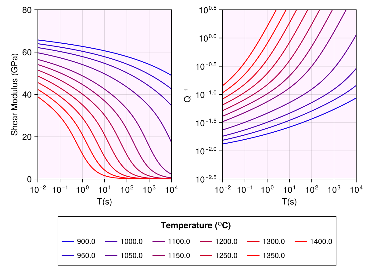
Analytical Andrade model
Porosity.andrade_analytical Type
andrade_analytical(T, P, dg, σ, ϕ, ρ, f)Calculate anelastic properties stored in RockPhyAnelastic using the Master curve maxwell scaling per McCarthy, Takei and Hiraga (2011)
Arguments
- `T` : Temperature of the rock (K)
- `P` : Pressure (GPa)
- `dg`: Grain size (μm)
- `σ` : Shear stress (GPa)
- `ϕ` : Porosity
- `ρ` : Density (kg/m³)
- `Ch2o_ol` : water concentration in olivine (in ppm), only used when using `HK2003` for viscosity calculations
- `T_solidus` : Solidus temperature (K), only used when using `xfit_premelt` for viscosity calculations
- `f` : frequency
Keyword Arguments
- `params` : Various coefficients required for calculation.
Also holds coefficients and the type of `RockphyElastic` model and `RockphyViscous model` to be used.

To investigate coefficients, call `default_params(Val{xfit_premelt}())`.
To modify coefficients, check the relevant documentation page. This
will also users to pick any particular type of `RockphyElastic` model, defaults to `anharmonic`,
as well as `RockphyViscous` model (for diffusion-derived viscosity), defaults to `HK2003`
Usage
Note
Make sure that the dimension of vector f is one more than the other parameters. Check relevant tutorials. Note the transpose on f when making the model in the following eg.
julia> T = [800, 1000] .+ 273.0f0;

julia> P = 2 .+ zero(T);

julia> dg = 4.0f0;

julia> σ = 10.0f-3;

julia> ϕ = 1.0f-2;

julia> ρ = 3300.0f0;

julia> Ch2o_ol = 0.0f0;

julia> T_solidus = 900 + 273.0f0;

julia> f = [1.0f0, 1.0f1];

julia> model = andrade_analytical(T, P, dg, σ, ϕ, ρ, Ch2o_ol, T_solidus, f')
Model : andrade_analytical
Temperature (K) : Float32[1073.0, 1273.0]
Pressure (GPa) : Float32[2.0, 2.0]
grain size(μm) : 4.0
Shear stress (GPa) : 0.01
Porosity : 0.01
Density (kg/m³) : 3300.0
Water concentration in olivine (ppm) : 0.0
Solidus Temperature (K) : 1173.0
Frequency (Hz) : Float32[1.0 10.0]

julia> forward(model, [])
Rock physics Response : RockphyAnelastic
Real part of dynamic compliance (Pa⁻¹) : Float32[1.3498141f-11 1.34976925f-11; 1.4012593f-11 1.4012127f-11]
Imaginary part of dynamic compliance (Pa⁻¹) : Float32[3.2687721f-16 1.5162017f-16; 6.353883f-16 1.8700414f-16]
Attenuation : Float32[2.4216462f-5 1.1233044f-5; 4.534409f-5 1.3345877f-5]
Modulus (Pa) : Float32[7.408428f10 7.4086736f10; 7.136438f10 7.1366754f10]
Anelastic S-wave velocity : (m/s) : Float32[4738.12 4738.1987; 4650.33 4650.4077]
Frequency averaged S-wave velocity (m/s) : Float32[4738.159, 4650.369]
References
Andrade, 1910, "On the viscous flow in metals, and allied phenomena", Proceedings of the Royal Society of London, https://doi.org/10.1098/rspa.1910.0050
Cooper, 2002, "Seismic Wave Attenuation: Energy Dissipation in Viscoelastic Crystalline Solids", Reviews in mineralogy and geochemistry, https://doi.org/10.2138/gsrmg.51.1.253,
Lau and Holtzman, 2019, "“Measures of Dissipation in Viscoelastic Media” Extended: Toward Continuous Characterization Across Very Broad Geophysical Time Scales", Geophysical Research Letters, https://doi.org/10.1029/2019GL083529
For different temperatures, the distribution with oscillation period looks like
Code for this figure
T = (900:50:1400) .+ 273.0
P = 0.2
dg = 3.1
σ = 10.0 * 1.0f-3
ϕ = 0.0
ρ = 3300.0
Ch2o_ol = 0.0
T_solidus = 1100 + 273.0

f = 10 .^ -collect(range(-2, 4; length=100))

m = andrade_analytical(T, P, dg, σ, ϕ, ρ, Ch2o_ol, T_solidus, f')

resp = forward(m, []);
size(resp.J1)

fig = Figure()
ax = Axis(fig[1, 1]; xscale=log10, backgroundcolor=(:magenta, 0.05),
    ylabel="Shear Modulus (GPa)", xlabel="T(s)")

for i in eachindex(T)
    color_ = RGBf(i / 10, 0.0, 1 - i / 10)
    lines!(ax, 1 ./ f, resp.M[i, :] ./ (1e9); color=color_, label="$(T[i] - 273)")
end
xlims!(ax, 1e-2, 1e4)
ylims!(ax, 0, 80)

ax2 = Axis(fig[1, 2]; xscale=log10, yscale=log10,
    backgroundcolor=(:magenta, 0.05), ylabel="Q⁻¹ ", xlabel="T(s)")

for i in eachindex(T)
    color_ = RGBf(i / 10, 0.0, 1 - i / 10)
    lines!(ax2, 1 ./ f, resp.Qinv[i, :]; color=color_, label="$(T[i] - 273)")
end
xlims!(ax2, 1e-2, 1e4)
ylims!(ax2, 10.0^(-2.5), 10.0^0.5)
fig[2, 1:2] = Legend(
    fig, ax, "Temperature (ᴼC) "; orientation=:horizontal, labelsize=12, nbanks=2)