Mixing phases

For various rock physics models, we require the bulk property by combing multiple phases. We allow the feature to mix multiple phases to get the bulk property.

Two phase models

Hashin-Shtrikman bounds, provided through HS1962_plus and HS1962_minus, are often used to estimate the bulk conductivity when two phases are mixed. For conductivity, modified Archie's law is also provided through MAL.

To get things started, we first need to define the phases we need to mix the models and the mixing law. This is conveniently done using two_phase_modelType

m = two_phase_modelType(Yoshino2009, Sifre2014, HS1962_plus)

two_phase_modelType{Yoshino2009, Sifre2014, HS1962_plus}(Yoshino2009, Sifre2014, HS1962_plus)

Now, we define the parameters required to define the model.

T = collect(1000:1400) .+ 273.0f0
Ch2o_ol = 1.0f0
Ch2o_m = 1000.0f0
Cco2_m = 10.0f0
ϕ = 0.1f0

ps_nt = (; ϕ=ϕ, T=T, Ch2o_ol=Ch2o_ol, Ch2o_m=Ch2o_m, Cco2_m=Cco2_m)
model = m(ps_nt)

and then as usual get the response

resp = forward(model, [])

and then plot :

Code for this figure

f = Figure()
ax = Axis(f[1, 1]; yscale=log10, xlabel="10⁴/T (K⁻¹)", ylabel="σ (S/m)",
    yticks=LogTicks(WilkinsonTicks(6; k_min=5)), backgroundcolor=(:magenta, 0.05))

xts = inv.([700, 900, 1100, 1300, 1500] .+ 273.0) .* 1e4

ax2 = Axis(f[1, 1]; yscale=log10, xaxisposition=:top, yaxisposition=:right, xlabel="T (ᴼC)",
    xgridvisible=false, xtickformat=x -> string.(round.((1e4 ./ x) .- 273)),
    xticklabelsize=10, backgroundcolor=(:magenta, 0.05))
ax2.xticks = xts
hidespines!(ax2)
hideydecorations!(ax2)
linkyaxes!(ax, ax2)

logsig = resp.σ

lines!(ax, inv.(T) .* 1e4, 10 .^ logsig)
lines!(ax2, inv.(T) .* 1e4, 10 .^ logsig; alpha=0)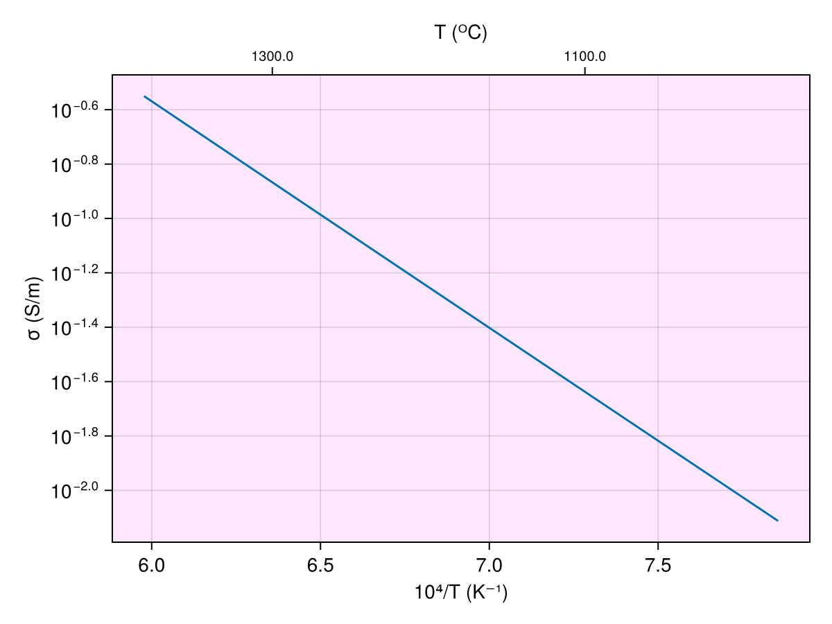

The above might seem complicated at the first sight but bears a very close analogy with the other rock physics types. Lets break it down bottom up :

• We had forward(model, []) similar to any other rock physics type, the last step to get the responses is to call the forward function.

• Before that, we had m(ps_nt) where ps_nt had the parameters. This looks very much like SEO3(1000. + 273) or anharmonic(T, P, ρ). Instead of passing the parameters as such, we now have to pass them through the NamedTuple called ps_nt because now, we do not know beforehand what parameters the mixed model will depend on. Had we used SEO3 with Gaillard2008, we would have only needed temperature (and obviously melt fraction).

• Before that, in the very first step, we had two_phase_modelType(Yoshino2009, Sifre2014, HS1962_plus()). Now, we do not have a comparison step here, but we do know that the output from this m is used in the similar fashion as SEO3, Yoshino2009 or Sifre2014. The two_phase_modelType function allows us to create one of these "types". For two phase mixing, we require the two phases along with the mixing law. Once we know them, we can completely define the physics at play, similar to how SEO3 or Yoshino2009 defines it in their way.

For different models, we have the distribution with melt fraction as (also a nice example of broadcasting) :

Code for this figure

T = collect(1000:100:1400) .+ 273.0f0
Ch2o_ol = 5.0f0
Ch2o_m = 1000.0f0
Cco2_m = 10.0f0
ϕ = (0.01f0:0.01f0:0.2f0)'

m = two_phase_modelType(Yoshino2009, Sifre2014, HS1962_plus)
ps_nt = (; ϕ=ϕ, T=T, Ch2o_ol=Ch2o_ol, Ch2o_m=Ch2o_m, Cco2_m=Cco2_m)
model = m(ps_nt)

sig1 = 10.0f0 .^ forward(model, []).σ

m = two_phase_modelType(Yoshino2009, Sifre2014, HS1962_minus)
ps_nt = (; ϕ=ϕ, T=T, Ch2o_ol=Ch2o_ol, Ch2o_m=Ch2o_m, Cco2_m=Cco2_m)
model = m(ps_nt)

sig2 = 10.0f0 .^ forward(model, []).σ

m = two_phase_modelType(Yoshino2009, Sifre2014, MAL)
ps_nt = (; ϕ=ϕ, T=T, Ch2o_ol=Ch2o_ol, Ch2o_m=Ch2o_m, Cco2_m=Cco2_m, m_MAL=1.2f0)
model = m(ps_nt)

sig3 = 10.0f0 .^ forward(model, []).σ

# plots

fig = Figure(; size=(900, 400))
ax1 = Axis(fig[1, 1]; yscale=log10, backgroundcolor=(:magenta, 0.05),
    ylabel="σ (S/m)", xlabel="ϕ", title="HS+ bound")

for i in eachindex(T)
    color_ = RGBf(i / 5, 0.0, 1 - i / 5)
    lines!(ax1, ϕ[:], sig1[i, :]; color=color_, label="$(T[i] - 273)")
end

ax2 = Axis(fig[1, 2]; yscale=log10, backgroundcolor=(:magenta, 0.05),
    ylabel="σ (S/m)", xlabel="T(s)", title="HS- bound")

for i in eachindex(T)
    color_ = RGBf(i / 5, 0.0, 1 - i / 5)
    lines!(ax2, ϕ[:], sig2[i, :]; color=color_, label="$(T[i] - 273)")
end

ax3 = Axis(fig[1, 3]; yscale=log10, backgroundcolor=(:magenta, 0.05),
    ylabel="σ (S/m)", xlabel="T(s)", title="Modified Archie's law")

for i in eachindex(T)
    color_ = RGBf(i / 5, 0.0, 1 - i / 5)
    lines!(ax3, ϕ[:], sig3[i, :]; color=color_, label="$(T[i] - 273)")
end

fig[2, 1:3] = Legend(fig, ax3, "Temperature (ᴼC)"; orientation=:horizontal, labelsize=12)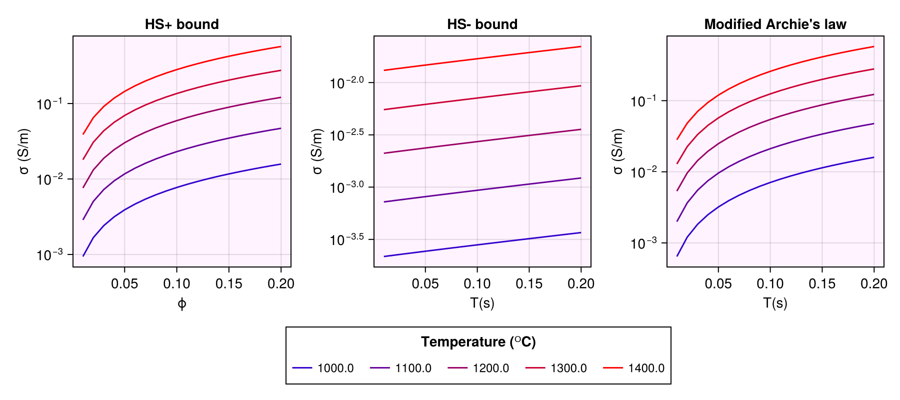

Info

Note that for [`MAL`](@ref), we need to provide cementation exponent, passed in through `ps_nt`

Multiple phase models

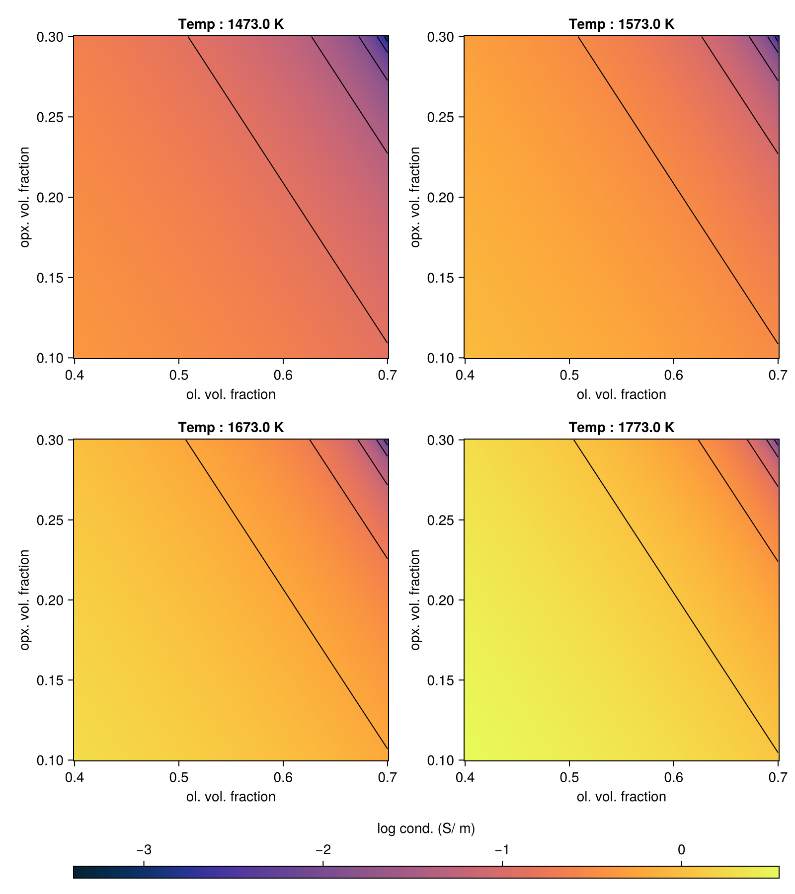
Multiple phases (upto 8) can be mixed using the Hashin-Shtrikman bounds for n-phases, HS_plus_multi_phase andHS_minus_multi_phase, and generalized Archie's law GAL.

For an example, let's define the parameters first :

T = [1200, 1300, 1400, 1500] .+ 273.0f0
Ch2o_ol = 5.0f0
Ch2o_opx = 20.0f0
Ch2o_m = 2000.0f0
Cco2_m = 10000.0f0
ϕ1 = (0.4f0:0.002f0:0.7f0)
ϕ2 = (0.1f0:0.001f0:0.3f0)

(T = Float32[1473.0, 1573.0, 1673.0, 1773.0], Ch2o_ol = 5.0f0, Ch2o_m = 2000.0f0, Cco2_m = 10000.0f0, ϕ = adjoint(0.01f0:0.01f0:0.2f0), Ch2o_opx = 20.0f0)

HS+

Code for this figure

m = multi_phase_modelType(UHO2014, Dai_Karato2009, Sifre2014, HS_plus_multi_phase)

logsig_mat = zeros(length(T), length(ϕ1), length(ϕ2))

for i in eachindex(ϕ1), j in eachindex(ϕ2)

    ϕ = [ϕ1[i], ϕ2[j]]
    ps_nt = (; ps_nt_..., ϕ)
    model = m(ps_nt)
    logsig_mat[:, i, j] .= forward(model, []).σ
end

fig = Figure(; size=(800, 900))
crange = extrema(logsig_mat)
cmap = :thermal
ax1 = Axis(fig[1, 1]; xlabel="ol. vol. fraction", ylabel="opx. vol. fraction", title="Temp : $(T[1]) K")
ax2 = Axis(fig[1, 2]; xlabel="ol. vol. fraction", ylabel="opx. vol. fraction", title="Temp : $(T[2]) K")
ax3 = Axis(fig[2, 1]; xlabel="ol. vol. fraction", ylabel="opx. vol. fraction", title="Temp : $(T[3]) K")
ax4 = Axis(fig[2, 2]; xlabel="ol. vol. fraction", ylabel="opx. vol. fraction", title="Temp : $(T[4]) K")

heatmap!(ax1, ϕ1, ϕ2, logsig_mat[1, :, :]; colorrange=crange, colormap=cmap)
contour!(ax1, ϕ1, ϕ2, logsig_mat[1, :, :]; color=:black)
heatmap!(ax2, ϕ1, ϕ2, logsig_mat[2, :, :]; colorrange=crange, colormap=cmap)
contour!(ax2, ϕ1, ϕ2, logsig_mat[2, :, :]; color=:black)
heatmap!(ax3, ϕ1, ϕ2, logsig_mat[3, :, :]; colorrange=crange, colormap=cmap)
contour!(ax3, ϕ1, ϕ2, logsig_mat[3, :, :]; color=:black)
h = heatmap!(ax4, ϕ1, ϕ2, logsig_mat[4, :, :]; colorrange=crange, colormap=cmap)
contour!(ax4, ϕ1, ϕ2, logsig_mat[4, :, :]; color=:black)
Colorbar(fig[3, :], h; vertical=false, label="log cond. (S/ m)")

┌ Warning: Assignment to `ϕ` in soft scope is ambiguous because a global variable by the same name exists: `ϕ` will be treated as a new local. Disambiguate by using `local ϕ` to suppress this warning or `global ϕ` to assign to the existing global variable.
└ @ mixing_phases.md:186
┌ Warning: Assignment to `ps_nt` in soft scope is ambiguous because a global variable by the same name exists: `ps_nt` will be treated as a new local. Disambiguate by using `local ps_nt` to suppress this warning or `global ps_nt` to assign to the existing global variable.
└ @ mixing_phases.md:187
┌ Warning: Assignment to `model` in soft scope is ambiguous because a global variable by the same name exists: `model` will be treated as a new local. Disambiguate by using `local model` to suppress this warning or `global model` to assign to the existing global variable.
└ @ mixing_phases.md:188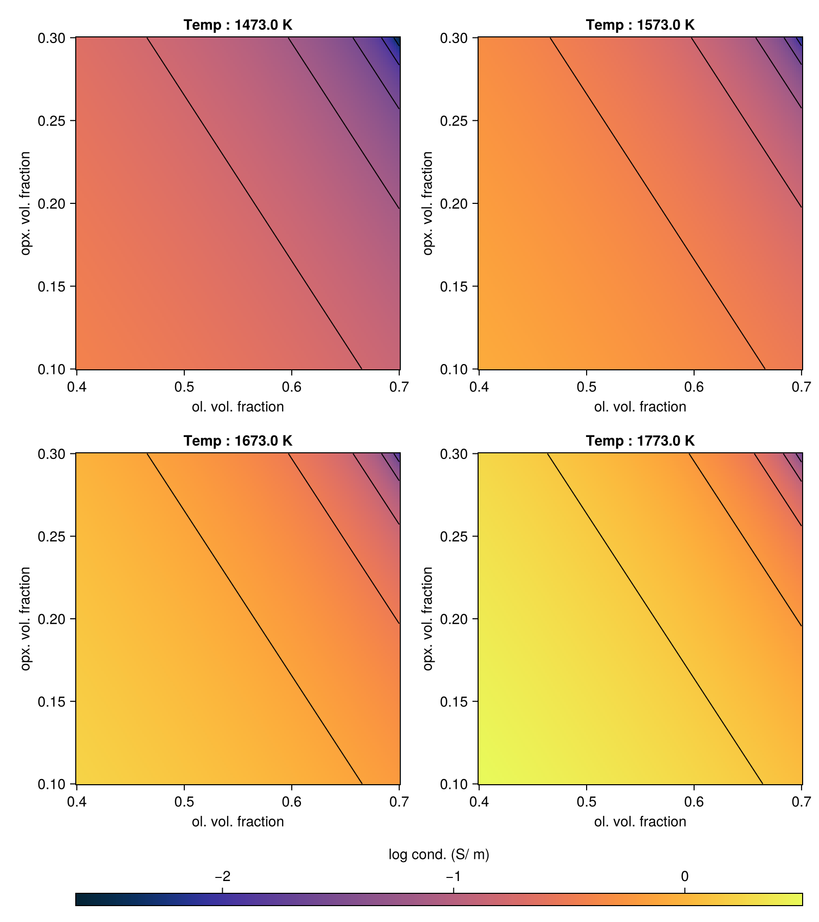

HS-

Code for this figure

m = multi_phase_modelType(UHO2014, Dai_Karato2009, Sifre2014, HS_minus_multi_phase)

logsig_mat = zeros(length(T), length(ϕ1), length(ϕ2))

for i in eachindex(ϕ1), j in eachindex(ϕ2)

    ϕ = [ϕ1[i], ϕ2[j]]
    ps_nt = (; ps_nt_..., ϕ)
    model = m(ps_nt)
    logsig_mat[:, i, j] .= forward(model, []).σ
end

fig = Figure(; size=(800, 900))
crange = extrema(logsig_mat)
cmap = :thermal
ax1 = Axis(fig[1, 1]; xlabel="ol. vol. fraction", ylabel="opx. vol. fraction", title="Temp : $(T[1]) K")
ax2 = Axis(fig[1, 2]; xlabel="ol. vol. fraction", ylabel="opx. vol. fraction", title="Temp : $(T[2]) K")
ax3 = Axis(fig[2, 1]; xlabel="ol. vol. fraction", ylabel="opx. vol. fraction", title="Temp : $(T[3]) K")
ax4 = Axis(fig[2, 2]; xlabel="ol. vol. fraction", ylabel="opx. vol. fraction", title="Temp : $(T[4]) K")

heatmap!(ax1, ϕ1, ϕ2, logsig_mat[1, :, :]; colorrange=crange, colormap=cmap)
contour!(ax1, ϕ1, ϕ2, logsig_mat[1, :, :]; color=:black)
heatmap!(ax2, ϕ1, ϕ2, logsig_mat[2, :, :]; colorrange=crange, colormap=cmap)
contour!(ax2, ϕ1, ϕ2, logsig_mat[2, :, :]; color=:black)
heatmap!(ax3, ϕ1, ϕ2, logsig_mat[3, :, :]; colorrange=crange, colormap=cmap)
contour!(ax3, ϕ1, ϕ2, logsig_mat[3, :, :]; color=:black)
h = heatmap!(ax4, ϕ1, ϕ2, logsig_mat[4, :, :]; colorrange=crange, colormap=cmap)
contour!(ax4, ϕ1, ϕ2, logsig_mat[4, :, :]; color=:black)
Colorbar(fig[3, :], h; vertical=false, label="log cond. (S/ m)")

┌ Warning: Assignment to `ϕ` in soft scope is ambiguous because a global variable by the same name exists: `ϕ` will be treated as a new local. Disambiguate by using `local ϕ` to suppress this warning or `global ϕ` to assign to the existing global variable.
└ @ mixing_phases.md:233
┌ Warning: Assignment to `ps_nt` in soft scope is ambiguous because a global variable by the same name exists: `ps_nt` will be treated as a new local. Disambiguate by using `local ps_nt` to suppress this warning or `global ps_nt` to assign to the existing global variable.
└ @ mixing_phases.md:234
┌ Warning: Assignment to `model` in soft scope is ambiguous because a global variable by the same name exists: `model` will be treated as a new local. Disambiguate by using `local model` to suppress this warning or `global model` to assign to the existing global variable.
└ @ mixing_phases.md:235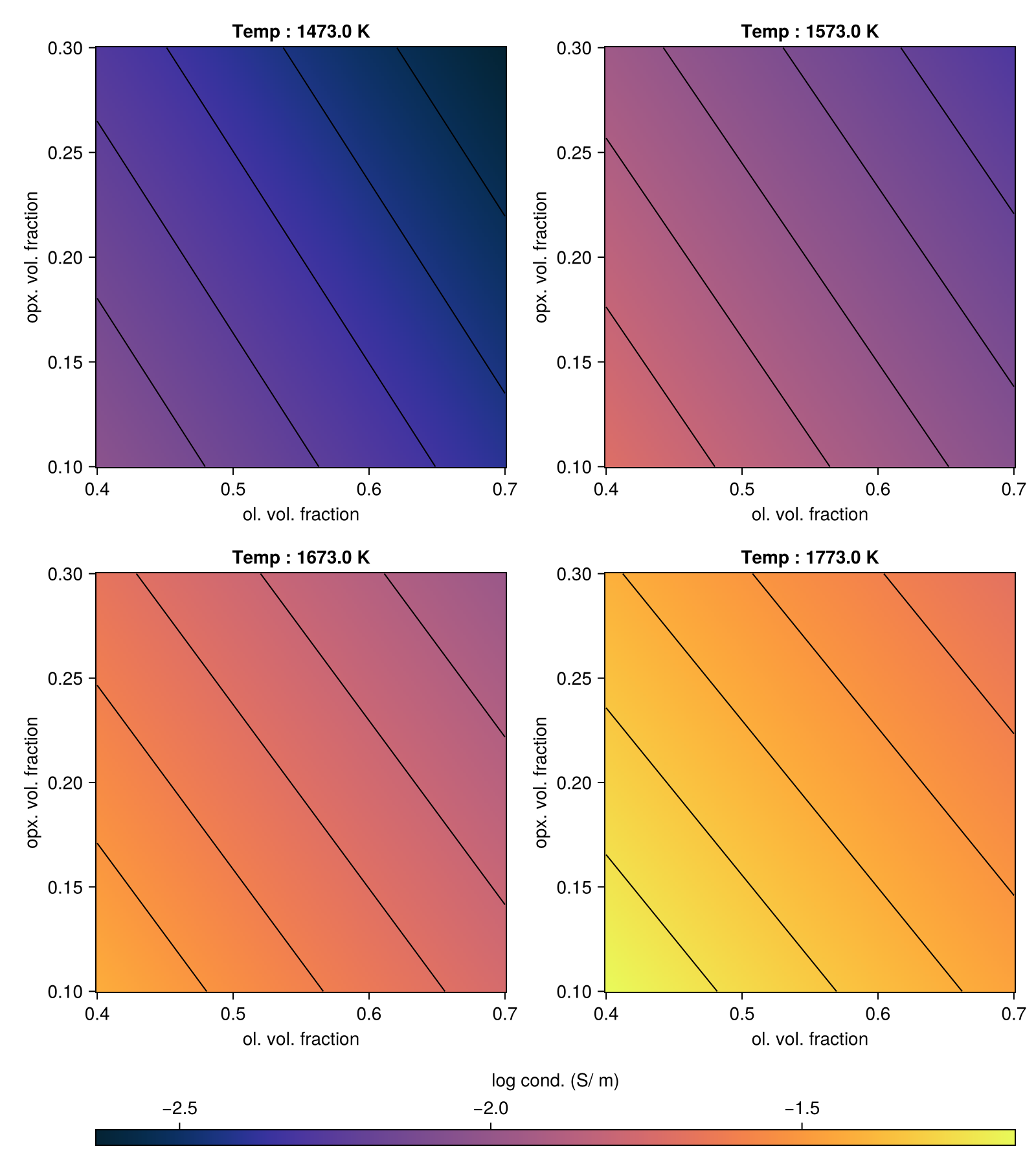

GAL

Info

Note that for [`GAL`](@ref), we need to provide cementation exponent, passed in through `ps_nt`

Code for this figure

m = multi_phase_modelType(UHO2014, Dai_Karato2009, Sifre2014, GAL)

logsig_mat = zeros(length(T), length(ϕ1), length(ϕ2))

for i in eachindex(ϕ1), j in eachindex(ϕ2)

    ϕ = [ϕ1[i], ϕ2[j]]
    ps_nt = (; ps_nt_..., ϕ, m_GAL=[5.0, 4.0, 1.2])
    model = m(ps_nt)
    logsig_mat[:, i, j] .= forward(model, []).σ
end

fig = Figure(; size=(800, 900))
crange = extrema(logsig_mat)
cmap = :thermal
ax1 = Axis(fig[1, 1]; xlabel="ol. vol. fraction", ylabel="opx. vol. fraction", title="Temp : $(T[1]) K")
ax2 = Axis(fig[1, 2]; xlabel="ol. vol. fraction", ylabel="opx. vol. fraction", title="Temp : $(T[2]) K")
ax3 = Axis(fig[2, 1]; xlabel="ol. vol. fraction", ylabel="opx. vol. fraction", title="Temp : $(T[3]) K")
ax4 = Axis(fig[2, 2]; xlabel="ol. vol. fraction", ylabel="opx. vol. fraction", title="Temp : $(T[4]) K")

heatmap!(ax1, ϕ1, ϕ2, logsig_mat[1, :, :]; colorrange=crange, colormap=cmap)
contour!(ax1, ϕ1, ϕ2, logsig_mat[1, :, :]; color=:black)
heatmap!(ax2, ϕ1, ϕ2, logsig_mat[2, :, :]; colorrange=crange, colormap=cmap)
contour!(ax2, ϕ1, ϕ2, logsig_mat[2, :, :]; color=:black)
heatmap!(ax3, ϕ1, ϕ2, logsig_mat[3, :, :]; colorrange=crange, colormap=cmap)
contour!(ax3, ϕ1, ϕ2, logsig_mat[3, :, :]; color=:black)
h = heatmap!(ax4, ϕ1, ϕ2, logsig_mat[4, :, :]; colorrange=crange, colormap=cmap)
contour!(ax4, ϕ1, ϕ2, logsig_mat[4, :, :]; color=:black)
Colorbar(fig[3, :], h; vertical=false, label="log cond. (S/ m)")

┌ Warning: Assignment to `ϕ` in soft scope is ambiguous because a global variable by the same name exists: `ϕ` will be treated as a new local. Disambiguate by using `local ϕ` to suppress this warning or `global ϕ` to assign to the existing global variable.
└ @ mixing_phases.md:284
┌ Warning: Assignment to `ps_nt` in soft scope is ambiguous because a global variable by the same name exists: `ps_nt` will be treated as a new local. Disambiguate by using `local ps_nt` to suppress this warning or `global ps_nt` to assign to the existing global variable.
└ @ mixing_phases.md:285
┌ Warning: Assignment to `model` in soft scope is ambiguous because a global variable by the same name exists: `model` will be treated as a new local. Disambiguate by using `local model` to suppress this warning or `global model` to assign to the existing global variable.
└ @ mixing_phases.md:286