Solvers from NonlinearSolve.jl

Brief introduction

We can solve the inverse problem using a suite of solvers provided by NonlinearSolve.jl such as :

• Gauss Newton

• Levenberg Marquardt

• Newton Raphson

Demo

Warning

Owing to the non-uniqueness of the geophysical methods, it might take considerable effort to obtain a model that converges and/or fits the data.

We demonstrate using Levenberg-Marquadt on a couple of geophysical models below:

Rayleigh waves

We first begin with an example for Rayleigh waves

Let's define a synthetic model:

vs = [3.2, 4.39731, 4.40192, 4.40653, 4.41113, 4.41574]
vp = [5.8, 8.01571, 7.99305, 7.97039, 7.94773, 7.92508]
ρ = [2.6, 3.38014, 3.37797, 3.37579, 3.37362, 3.37145]
h = [20.0, 20.0, 20.0, 20.0, 20.0] .* 1e3
m = RWModel(vs, h, ρ, vp)

1D Rayleigh Wave Model
┌───────┬────────┬──────────┬───────────┬──────────┬────────┐
│ Layer │     vₛ │        h │         z │        ρ │     vₚ │
│       │ [km/s] │      [m] │       [m] │ [kg⋅m⁻³] │ [km/s] │
├───────┼────────┼──────────┼───────────┼──────────┼────────┤
│     1 │   3.20 │ 20000.00 │  20000.00 │      2.6 │    5.8 │
│     2 │   4.40 │ 20000.00 │  40000.00 │     3.38 │  8.016 │
│     3 │   4.40 │ 20000.00 │  60000.00 │    3.378 │  7.993 │
│     4 │   4.41 │ 20000.00 │  80000.00 │    3.376 │   7.97 │
│     5 │   4.41 │ 20000.00 │ 100000.00 │    3.374 │  7.948 │
│     6 │   4.42 │        ∞ │         ∞ │    3.371 │  7.925 │
└───────┴────────┴──────────┴───────────┴──────────┴────────┘

and then get the forward response, with 1% error floors :

freq = exp10.(-2:0.1:1)
t = inv.(freq)

resp = forward(m, t)

err_resp = SurfaceWaveResponse(0.01 .* resp.c,)

SurfaceWaveResponse{Vector{Float64}}([0.03998742809891676, 0.039827418196201086, 0.03964482211470581, 0.039434630930423514, 0.039178924423455976, 0.038826487535238055, 0.03824804467558841, 0.03714191050529463, 0.035061089980602145, 0.03253521530628197  …  0.02958232079744337, 0.02958232079744337, 0.02958232079744337, 0.029582320785522444, 0.029582320785522444, 0.029582320785522444, 0.029582320785522444, 0.029582320785522444, 0.029582320785522444, 0.029582320785522444])

We need to define a data covariance matrix $C_d$ and an initial model. Let's assume gaussian noise in this case, and choose an initial model a half-space of 100 $\mathrm{\Omega }m$.

h_test = fill(2500.0, 50)
m_lm = RWModel(4.0 .+ zeros(length(h_test) + 1), h_test, fill(3e3, 51), fill(7e3, 51))

C_d = diagm(inv.(err_resp.c)) .^ 2

The final result will be stored in the same variable m_occam. All we need to do now is specify using Occam and then calling inverse!.

Note

Using Occam, you also have the option to perform a smoothing step. Once the model has achieved the threshold misfit, it is smoothened until it fits the data just about the threshold misfit.

alg_cache = NonlinearAlg(; alg=LevenbergMarquardt(; autodiff=AutoFiniteDiff()), μ=100.0)
rw_bounds = transform_utils(
    x -> SubsurfaceCore.sigmoid(x, 3.0, 5.0), x -> SubsurfaceCore.inverse_sigmoid(x, 3.0, 5.0))
C_m = Float64.(I(51))
retcode = inverse!(
    m_lm, resp, t, alg_cache; W=C_d, max_iters=100, verbose=10, model_trans_utils=rw_bounds);

iteration = 10 : data misfit => 24.016793429299955
iteration = 20 : data misfit => 21.367215706965634
iteration = 30 : data misfit => 21.386778986769137
iteration = 40 : data misfit => 20.638007752085624
iteration = 50 : data misfit => 17.266549218602318
iteration = 60 : data misfit => 15.578266439796748
iteration = 70 : data misfit => 13.879451065487975
iteration = 80 : data misfit => 12.482374310416184
iteration = 90 : data misfit => 11.087144184845759
iteration = 100 : data misfit => 9.886717400936815

Code for this figure

fig = Figure()
ax_m = Axis(fig[1, 1]; xlabel="Vs (km/s)", ylabel="depth (m)")

plot_model!(ax_m, m; label="true", color=:steelblue3)
plot_model!(ax_m, m_lm; label="occam", color=:tomato)
fig

ax1 = Axis(fig[1, 2]; xscale=log10)

plot_response!([ax1], t, resp; plt_type=:scatter, color=:steelblue3)
plot_response!(
    [ax1], t, resp; errs=err_resp, plt_type=:errors, whiskerwidth=10, color=:steelblue3)

resp_lm = forward(m_lm, t)
plot_response!([ax1], t, resp_lm; color=:tomato)
Legend(fig[2, :], ax_m; orientation=:horizontal)
fig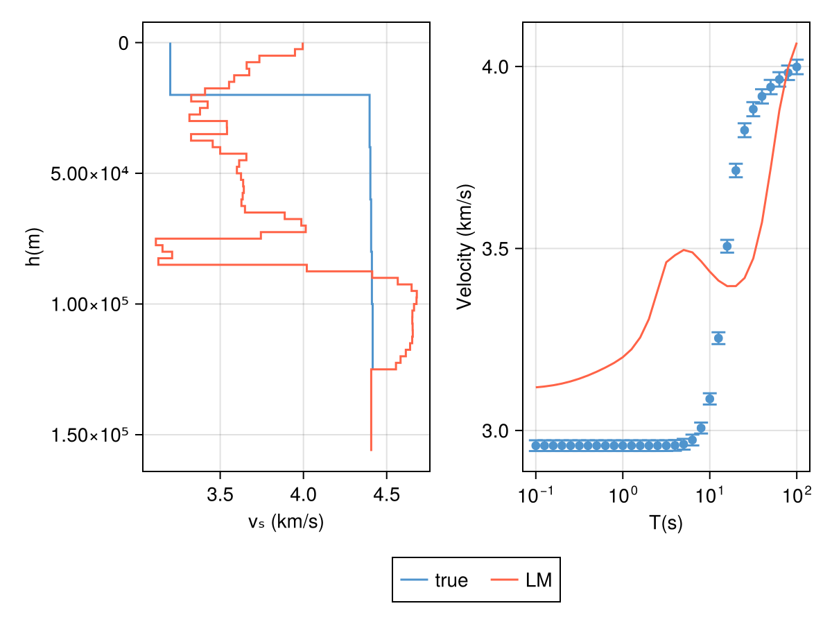

This one did not converge, and that's geophysical inversion 90% of the time. 😃

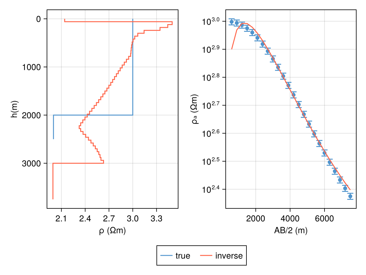
DC Resistivity

Let's try and see if we can get things to converge for a simple DC resistivity model. Let's make another synthetic model with 5 % error floors for Wenner array.

ρ = log10.([1000.0, 100.0])
h = [2000.0]
m = DCModel(ρ, h)

locs = get_wenner_array(400:200:5000)
resp = forward(m, locs)

err_resp = DCResponse(0.05 .* resp.ρₐ)

DCResponse{Vector{Float64}}([49.78080378133154, 49.29938773593118, 48.44937258369504, 47.20042003213615, 45.577483232511035, 43.63801768288286, 41.457587555509846, 39.11689974493678, 36.69228868217137, 34.2502534693876  …  23.26586758159128, 21.46552117101448, 19.81179059476642, 18.301934999175476, 16.93084667959415, 15.691352796166434, 14.57172215520599, 13.560689085508915, 12.654629590939471, 11.854125017539744])

Now, defining an initial model and covariance matrix:

h_test = fill(60.0, 50)
m_lm = DCModel(2.0 .+ zeros(length(h_test) + 1), h_test)

C_d = diagm(inv.(err_resp.ρₐ)) .^ 2

and then

alg_cache = NonlinearAlg(; alg=LevenbergMarquardt(; autodiff=AutoFiniteDiff()), μ=10.0)
retcode = inverse!(m_lm, resp, locs, alg_cache; W=C_d, max_iters=100);

iteration = 1 : data misfit => 15.971069578258938
iteration = 2 : data misfit => 15.971069578258938
iteration = 3 : data misfit => 15.971069578258938
iteration = 4 : data misfit => 15.971069578258938
iteration = 5 : data misfit => 15.971069578258938
iteration = 6 : data misfit => 15.971069578258938
iteration = 7 : data misfit => 15.971069578258938
iteration = 8 : data misfit => 15.971069578258938
iteration = 9 : data misfit => 15.971069578258938
iteration = 10 : data misfit => 15.971069578258938
iteration = 11 : data misfit => 15.197976055250257
iteration = 12 : data misfit => 13.176768101044258
iteration = 13 : data misfit => 9.87295982297597
iteration = 14 : data misfit => 9.87295982297597
iteration = 15 : data misfit => 9.03423014707974
iteration = 16 : data misfit => 9.03423014707974
iteration = 17 : data misfit => 9.03423014707974
iteration = 18 : data misfit => 8.016350568771163
iteration = 19 : data misfit => 6.510958068881692
iteration = 20 : data misfit => 6.510958068881692
iteration = 21 : data misfit => 6.510958068881692
iteration = 22 : data misfit => 5.494525229239119
iteration = 23 : data misfit => 4.28680496092325
iteration = 24 : data misfit => 4.28680496092325
iteration = 25 : data misfit => 4.28680496092325
iteration = 26 : data misfit => 4.28680496092325
iteration = 27 : data misfit => 3.596760838741788
iteration = 28 : data misfit => 2.881323255851079
iteration = 29 : data misfit => 2.0077036675465734
iteration = 30 : data misfit => 1.2872081528323651
iteration = 31 : data misfit => 1.2872081528323651
iteration = 32 : data misfit => 1.2872081528323651
iteration = 33 : data misfit => 1.1297065426319755
iteration = 34 : data misfit => 1.1297065426319755
iteration = 35 : data misfit => 1.1297065426319755
iteration = 36 : data misfit => 1.0359178664017255
iteration = 37 : data misfit => 1.0359178664017255
iteration = 38 : data misfit => 0.9905317620425997

Code for this figure

fig = Figure()
ax_m = Axis(fig[1, 1])

plot_model!(ax_m, m; label="true", color=:steelblue3)
plot_model!(ax_m, m_lm; label="inverse", color=:tomato)
fig

ax1 = Axis(fig[1, 2]; xscale=log10)

ab_2 = abs.(locs.srcs[:, 2] .- locs.srcs[:, 1]) ./ 2
plot_response!([ax1], ab_2, resp; plt_type=:scatter, color=:steelblue3)
plot_response!(
    [ax1], ab_2, resp; errs=err_resp, plt_type=:errors, whiskerwidth=10, color=:steelblue3)

resp_lm = forward(m_lm, locs)
plot_response!([ax1], ab_2, resp_lm; color=:tomato)
Legend(fig[2, :], ax_m; orientation=:horizontal)
fig