PrISM.jl

RTO-TKO

RTO-TKO is a stochastic framework introduced in the electromagnetic geophysical community by Blatter et al., 2022 (a and b)

Similar to fixed discretization scheme, the grid sizes do not change. RTO-TKO tries to obtain the samples of the posterior distribution by unrolling the optimization for the misfit function, that is, it perturbs the model space obtained after one iteration before optimizing for the next. It does this iteratively for both the values of the model space and the regularization coefficient in alternative steps.

Therefore, if we have

m = [m_{1}, m_{2}, m_{3}, . . ., m_{N}]

and

d = F (m)

Then for $C_{d}$ , the inverse of data covariance matrix, and $C_{m}$ the inverse of model covariance matrix, we want to explore uncertainty for the following misfit function:

J (m) = [F (m) - d]^{T} C_{d} [F (m) - d] + μ m^{T} C_{m} m

where $μ$ is the regularization weight and $L$ is the derivative matrix. Probabilistically, the above equation implies that the a priori distribution of $m$ is $N (0, C_{m})$ . RTO-TKO explores the uncertainty in $m$ , as well as the $μ$ -space instead of fixing it, and gives a family of models that fit the data.

The algorithm was proposed for $C_{m}$ constructed with $L^{'} L$ , where $L$ is the discrete derivative matrix. The algorithm works as:

\begin{aligned} Solving for \\ J (m) = [F (m) - d]^{T} C_{d} [F (m) - d] + μ (L m)^{T} (L m) \\ 1) Solve for m_{i + 1} \\ Sample \tilde{d} \sim N (d, C_{d}) and \tilde{m} \sim N (0, \frac{1}{μ} (L^{T} L)) \\ Solve \\ m_{i + 1} = \argmin_{m_{i + 1}} [F (m_{i + 1}) - \tilde{d}]^{T} C_{d} [F (m_{i + 1}) - \tilde{d}] + μ_{i} [L (m_{i + 1} - \tilde{m})]^{T} [L (m_{i + 1} - \tilde{m})] \\ 2) Solve for μ_{i + 1} \\ Sample \tilde{d} \sim N (d, C_{d}) \\ Solve \\ μ_{i + 1} = \argmin_{μ_{i + 1}} [F (m_{i + 1}) - \tilde{d}]^{T} C_{d} [F (m_{i + 1}) - \tilde{d}] - l o g (p (μ_{i + 1})) \end{aligned}

Note

Usually, the prior of $μ$ is a uniform distribution and we do not have to compute the corresponding log pdf term
Implementing the above from scratch might not be trivial because of $L^{'} L$ being non-invertible, and we do the optimization in the domain defined by $ξ = \sqrt{μ} L m$ . Such a variable will then have a standard normal distribution $N (0, I)$ when $m \sim N (0, \frac{1}{μ} (L^{T} L))$

In the following section, we demonstrate RTO-TKO for a 6-layered earth, including the half-space being imaged using the MT method. The prior distribution is composed of 26 layers, with the initial model being a half-space.

Demo

Let's create a synthetic dataset first, with 10% error floors:

julia

m_test = MTModel(log10.([100.0, 10.0, 1000.0]), [1e3, 1e3])
f = 10 .^ range(-4; stop=1, length=25)
ω = vec(2π .* f)

r_obs = forward(m_test, ω)

err_phi = asin(0.02) * 180 / π .* ones(length(ω))
err_appres = 0.1 * r_obs.ρₐ
err_resp = MTResponse(err_appres, err_phi)

We don't need to construct the a priori the same way as before. Instead, we need to define the optimiser we'd use. Here, we use Occam, and an initial model composed of half-space of 100 $Ω m$ .

julia

z = collect(0:100:2.5e3)
h = diff(z)
m_rto = MTModel(2 .* ones(length(z)), vec(h))

n_samples = 100

r_cache = rto_cache(
    m_rto, [1e-2, 1e4], Occam(), n_samples, n_samples, 1.0, [:ρₐ, :ϕ], false)

rto_chain = stochastic_inverse(
    r_obs, err_resp, ω, r_cache; model_trans_utils=(; m=sigmoid_tf))

Chains MCMC chain (99×27×1 reshape(adjoint(::Matrix{Float64}), 99, 27, 1) with eltype Float64):

Iterations        = 1:1:99
Number of chains  = 1
Samples per chain = 99
parameters        = m[1], m[2], m[3], m[4], m[5], m[6], m[7], m[8], m[9], m[10], m[11], m[12], m[13], m[14], m[15], m[16], m[17], m[18], m[19], m[20], m[21], m[22], m[23], m[24], m[25], m[26], m[27]

Summary Statistics
  parameters      mean       std      mcse   ess_bulk   ess_tail      rhat   e ⋯
      Symbol   Float64   Float64   Float64    Float64    Float64   Float64     ⋯

        m[1]    1.9726    0.3050    0.1503     3.7949    15.2077    1.2015     ⋯
        m[2]    1.9542    0.3374    0.1978     2.7744    17.7102    1.3199     ⋯
        m[3]    1.8998    0.3124    0.1635     3.8949    15.2013    1.2032     ⋯
        m[4]    1.8476    0.3506    0.1974     3.0296    20.6296    1.2861     ⋯
        m[5]    1.7278    0.2794    0.1185     5.8540    21.2053    1.1287     ⋯
        m[6]    1.6914    0.3484    0.1507     7.0283    20.1674    1.1353     ⋯
        m[7]    1.6076    0.3008    0.1377     5.3998    54.8954    1.1427     ⋯
        m[8]    1.5018    0.2710    0.1276     3.7869    30.0359    1.2186     ⋯
        m[9]    1.3680    0.2785    0.0521    30.7837    37.6522    1.0482     ⋯
       m[10]    1.2938    0.2955    0.1028     8.1414    47.1088    1.0991     ⋯
       m[11]    1.1946    0.2908    0.0220   174.5857    85.9151    0.9937     ⋯
       m[12]    1.1510    0.2658    0.0473    30.3417    23.1605    1.0337     ⋯
       m[13]    1.0771    0.3322    0.0957    16.1218    72.1426    1.0703     ⋯
       m[14]    1.0548    0.2970    0.0675    22.6754    17.3669    1.0048     ⋯
       m[15]    1.1021    0.2583    0.0794     9.7461    45.9151    1.0836     ⋯
       m[16]    1.2009    0.3070    0.1352     5.0883    59.2731    1.1540     ⋯
       m[17]    1.2659    0.3000    0.1405     4.6987    91.3199    1.1675     ⋯
      ⋮           ⋮         ⋮         ⋮         ⋮          ⋮          ⋮        ⋱
                                                    1 column and 10 rows omitted

Quantiles
  parameters      2.5%     25.0%     50.0%     75.0%     97.5% 
      Symbol   Float64   Float64   Float64   Float64   Float64 

        m[1]    1.2559    1.8230    1.9957    2.1489    2.4950
        m[2]    1.2650    1.7900    1.9711    2.1811    2.5544
        m[3]    1.1771    1.7523    1.9295    2.1145    2.3709
        m[4]    1.1390    1.6055    1.8781    2.1152    2.3894
        m[5]    1.0595    1.5367    1.7652    1.8862    2.1482
        m[6]    0.9575    1.5487    1.7719    1.8996    2.2137
        m[7]    0.9628    1.4546    1.6382    1.7799    2.0680
        m[8]    0.9258    1.3693    1.5442    1.7021    1.9369
        m[9]    0.7699    1.2338    1.3909    1.5432    1.8113
       m[10]    0.7657    1.0877    1.2879    1.5148    1.8667
       m[11]    0.7034    0.9747    1.1638    1.4496    1.6928
       m[12]    0.6346    0.9860    1.1379    1.3695    1.6424
       m[13]    0.4839    0.8480    1.0637    1.2910    1.8066
       m[14]    0.5619    0.8425    1.0291    1.2442    1.7386
       m[15]    0.6842    0.8788    1.1201    1.2824    1.6200
       m[16]    0.6740    1.0035    1.1787    1.3961    1.8491
       m[17]    0.6793    1.0487    1.2393    1.4763    1.8009
      ⋮           ⋮         ⋮         ⋮         ⋮         ⋮
                                                 10 rows omitted

Since RTO-TKO also samples the regularization coefficient along with model parameters, we exclude it to obtain another chain as:

julia

mt_chain = Chains((rto_chain.value.data[:, 1:(end - 1), :]), [Symbol("m[$i]")
                                                              for i in 1:length(z)])

Chains MCMC chain (99×26×1 Array{Float64, 3}):

Iterations        = 1:1:99
Number of chains  = 1
Samples per chain = 99
parameters        = m[1], m[2], m[3], m[4], m[5], m[6], m[7], m[8], m[9], m[10], m[11], m[12], m[13], m[14], m[15], m[16], m[17], m[18], m[19], m[20], m[21], m[22], m[23], m[24], m[25], m[26]

Summary Statistics
  parameters      mean       std      mcse   ess_bulk   ess_tail      rhat   e ⋯
      Symbol   Float64   Float64   Float64    Float64    Float64   Float64     ⋯

        m[1]    1.9726    0.3050    0.1503     3.7949    15.2077    1.2015     ⋯
        m[2]    1.9542    0.3374    0.1978     2.7744    17.7102    1.3199     ⋯
        m[3]    1.8998    0.3124    0.1635     3.8949    15.2013    1.2032     ⋯
        m[4]    1.8476    0.3506    0.1974     3.0296    20.6296    1.2861     ⋯
        m[5]    1.7278    0.2794    0.1185     5.8540    21.2053    1.1287     ⋯
        m[6]    1.6914    0.3484    0.1507     7.0283    20.1674    1.1353     ⋯
        m[7]    1.6076    0.3008    0.1377     5.3998    54.8954    1.1427     ⋯
        m[8]    1.5018    0.2710    0.1276     3.7869    30.0359    1.2186     ⋯
        m[9]    1.3680    0.2785    0.0521    30.7837    37.6522    1.0482     ⋯
       m[10]    1.2938    0.2955    0.1028     8.1414    47.1088    1.0991     ⋯
       m[11]    1.1946    0.2908    0.0220   174.5857    85.9151    0.9937     ⋯
       m[12]    1.1510    0.2658    0.0473    30.3417    23.1605    1.0337     ⋯
       m[13]    1.0771    0.3322    0.0957    16.1218    72.1426    1.0703     ⋯
       m[14]    1.0548    0.2970    0.0675    22.6754    17.3669    1.0048     ⋯
       m[15]    1.1021    0.2583    0.0794     9.7461    45.9151    1.0836     ⋯
       m[16]    1.2009    0.3070    0.1352     5.0883    59.2731    1.1540     ⋯
       m[17]    1.2659    0.3000    0.1405     4.6987    91.3199    1.1675     ⋯
      ⋮           ⋮         ⋮         ⋮         ⋮          ⋮          ⋮        ⋱
                                                     1 column and 9 rows omitted

Quantiles
  parameters      2.5%     25.0%     50.0%     75.0%     97.5% 
      Symbol   Float64   Float64   Float64   Float64   Float64 

        m[1]    1.2559    1.8230    1.9957    2.1489    2.4950
        m[2]    1.2650    1.7900    1.9711    2.1811    2.5544
        m[3]    1.1771    1.7523    1.9295    2.1145    2.3709
        m[4]    1.1390    1.6055    1.8781    2.1152    2.3894
        m[5]    1.0595    1.5367    1.7652    1.8862    2.1482
        m[6]    0.9575    1.5487    1.7719    1.8996    2.2137
        m[7]    0.9628    1.4546    1.6382    1.7799    2.0680
        m[8]    0.9258    1.3693    1.5442    1.7021    1.9369
        m[9]    0.7699    1.2338    1.3909    1.5432    1.8113
       m[10]    0.7657    1.0877    1.2879    1.5148    1.8667
       m[11]    0.7034    0.9747    1.1638    1.4496    1.6928
       m[12]    0.6346    0.9860    1.1379    1.3695    1.6424
       m[13]    0.4839    0.8480    1.0637    1.2910    1.8066
       m[14]    0.5619    0.8425    1.0291    1.2442    1.7386
       m[15]    0.6842    0.8788    1.1201    1.2824    1.6200
       m[16]    0.6740    1.0035    1.1787    1.3961    1.8491
       m[17]    0.6793    1.0487    1.2393    1.4763    1.8009
      ⋮           ⋮         ⋮         ⋮         ⋮         ⋮
                                                  9 rows omitted

Note that the chain contains fewer samples than we had asked for. This is because a few unstable samples were filtered out. The obtained mt_chain contains the a posteriori distributions that can be saved using JLD2.jl.

julia

using JLD2
JLD2.@save "file_path.jld2" mt_chain

Since RTO-TKO is closely related to Occam, we also include occam results in our figures below. Also, note that we did not require an a priori distribution to obtain samples. However, we would need to create the same to plot our posterior samples. This can just be something that encapsulates the whole prior space (or an envelope of the same), e.g., in the case of magnetotelluric imaging, we know that the resistivity values will always be in [-2, 5] on the log-scale.

julia

modelD = MTModelDistribution(Product([Uniform(-1.0, 5.0) for i in eachindex(z)]), vec(h))

Code for this figure

julia

fig = Figure()
ax = Axis(fig[1, 1])
hm = get_kde_image!(ax, mt_chain, modelD; kde_transformation_fn=log10,
    colormap=:binary, colorrange=(-3.0, 0.0), trans_utils=(m=no_tf, h=no_tf))
Colorbar(fig[1, 2], hm; label="log pdf")

mean_kws = (; color=:seagreen3, linewidth=2)
std_kws = (; color=:red, linewidth=1.5)
# get_mean_std_image!(ax, mt_chain, modelD; confidence_interval=0.99, trans_utils=(m=no_tf, h=no_tf), mean_kwargs=mean_kws,
#     std_plus_kwargs=std_kws, std_minus_kwargs=std_kws)
ylims!(ax, [2500, 0])

plot_model!(ax, m_test; color=:black, linestyle=:dash, label="true", linewidth=2)
Legend(fig[2, :], ax; orientation=:horizontal)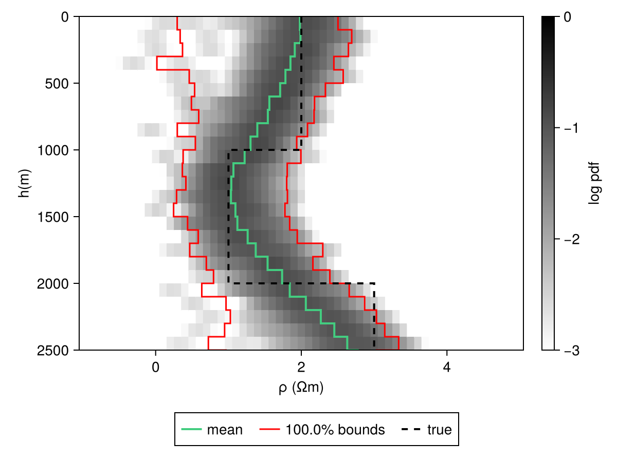

The list of models can then be obtained from chains using

julia

model_list = get_model_list(mt_chain, modelD)

We can then easily check the fit of the response curves

julia

fig = Figure()
ax1 = Axis(fig[1, 1])
ax2 = Axis(fig[1, 2])

resp_post = forward(model_list[1], ω);
for i in 1:(length(model_list) > 100 ? 100 : length(model_list))
    forward!(resp_post, model_list[i], ω)
    plot_response!([ax1, ax2], ω, resp_post; alpha=0.4, color=:gray)
end
plot_response!([ax1, ax2], ω, r_obs; errs=err_resp, plt_type=:errors, whiskerwidth=10)
plot_response!([ax1, ax2], ω, r_obs; plt_type=:scatter, label="true")
ylims!(ax1, exp10.([1.2, 3.1]))
ylims!(ax2, [12, 70])

fig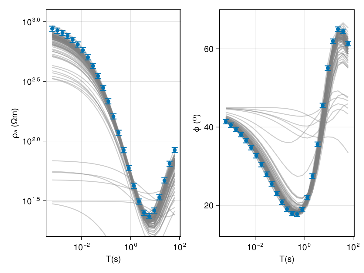

Warning

It is recommended that the samples from RTO-TKO can be filtered out to reject the samples that have a poor fit on the data.

RTO-TKO ​

Demo ​

RTO-TKO

Demo