Magnetotellurics (MT)

Model

We assume the following subsurface resistivity distribution with 4 layers:

Layer #	thickness (m)	$\rho (\mathrm{\Omega }m$)
1	1000	500
2	2000	1000
3	200	10
4	$\mathrm{\infty }$	100

The MTModel is defined as :

ρ = log10.([500.0, 1000.0, 10.0, 100.0])
h = [1000.0, 2000.0, 200.0]
m = MTModel(ρ, h)

1D MT Model
┌───────┬───────┬─────────┬─────────┐
│ Layer │ log-ρ │       h │       z │
│       │  [Ωm] │     [m] │     [m] │
├───────┼───────┼─────────┼─────────┤
│     1 │  2.70 │ 1000.00 │ 1000.00 │
│     2 │  3.00 │ 2000.00 │ 3000.00 │
│     3 │  1.00 │  200.00 │ 3200.00 │
│     4 │  2.00 │       ∞ │       ∞ │
└───────┴───────┴─────────┴─────────┘

Code for this figure

fig = Figure()
ax = Axis(fig[1, 1]; xlabel="log ρ (Ωm)", ylabel="depth (m)", backgroundcolor=(
    :magenta, 0.05))

plot_model!(ax, m)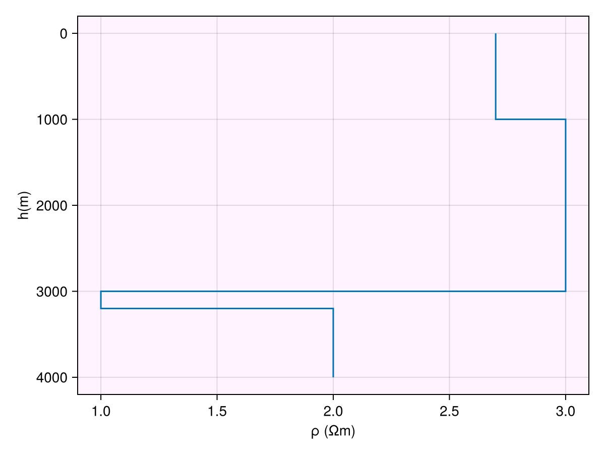

Warn

Always use Float64 or Float32 types while defining the vectors for resistivity and thickness. Using Int will throw an InexactError, e.g. : InexactError: Int64(4193.453970907305)

Response

To obtain the responses, that is apparent resistivity ρₐ and phase ϕ, we first need to define the frequencies :

freq = exp10.(-2:0.2:4)
ω = 2π .* freq
T = inv.(freq)

31-element Vector{Float64}:
 100.0
  63.09573444801933
  39.810717055349734
  25.118864315095795
  15.848931924611133
  10.0
   6.3095734448019325
   3.9810717055349727
   2.51188643150958
   1.5848931924611134
   ⋮
   0.003981071705534973
   0.0025118864315095794
   0.001584893192461114
   0.001
   0.000630957344480193
   0.0003981071705534973
   0.00025118864315095795
   0.0001584893192461114
   0.0001

and then call the forward dispatch and get MTResponse:

resp = forward(m, ω)

Code for this figure

fig = Figure() #size = (800, 600))
ax1 = Axis(fig[1, 1]; backgroundcolor=(:magenta, 0.05), aspect=AxisAspect(1))
ax2 = Axis(fig[1, 2]; backgroundcolor=(:magenta, 0.05), aspect=AxisAspect(1))

plot_response!([ax1, ax2], T, resp; plt_type=:scatter)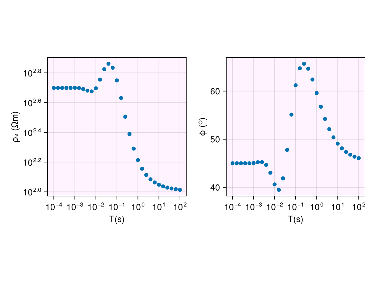

In-place operations

Mutating forward calls are also supported. This leads to no extra allocations while calculating the forward responses. This also speeds up the performance, though the calculations in the well-optimized forward calls are way more expensive than allocations to get a significant boost here. We now call the in-place variant forward! and provide an MTResponse variable to be overwritten :

forward!(resp, m, ω)

We can compare the allocations made in the two calls:

@allocated forward!(resp, m, ω)

0

@allocated forward(m, ω)

640

Benchmarks

While the exact runtimes will vary across processors, the runtimes increase linearly with number of layers.

Benchmark code

n_layers = Int.(exp2.(2:1:6))
freq = exp10.(-2:0.2:4)
ω = 2π .* freq

btime_iip = Float64.(zero(n_layers))
btime_oop = Float64.(zero(n_layers))
for i in eachindex(n_layers)
    ρ = 2 .* randn(n_layers[i])
    h = 100 .* rand(n_layers[i]-1)
    m = MTModel(ρ, h)
    resp = forward(m, ω)
    time_oop = @timed begin
        for i in 1:1000
            forward(m, ω)
        end
    end
    btime_oop[i] = time_oop.time/1e3
    forward!(resp, m, ω)
    time_iip = @timed begin
        for i in 1:1000
            forward!(resp, m, ω)
        end
    end
    btime_iip[i] = time_iip.time/1e3
end

fig = Figure()
ax = Axis(fig[1, 1]; xscale=log2, backgroundcolor=(:magenta, 0.05),
    xlabel="no. of layers", ylabel="time (ms)")
lines!(n_layers, btime_oop .* 1e3; label="out-of place forward calls", color=:tomato)
lines!(n_layers, btime_iip .* 1e3; label="in place forward calls",
    linestyle=:dash, color=:steelblue3)
Legend(fig[1, 2], ax)

┌ Warning: Assignment to `ρ` in soft scope is ambiguous because a global variable by the same name exists: `ρ` will be treated as a new local. Disambiguate by using `local ρ` to suppress this warning or `global ρ` to assign to the existing global variable.
└ @ mt.md:124
┌ Warning: Assignment to `h` in soft scope is ambiguous because a global variable by the same name exists: `h` will be treated as a new local. Disambiguate by using `local h` to suppress this warning or `global h` to assign to the existing global variable.
└ @ mt.md:125
┌ Warning: Assignment to `m` in soft scope is ambiguous because a global variable by the same name exists: `m` will be treated as a new local. Disambiguate by using `local m` to suppress this warning or `global m` to assign to the existing global variable.
└ @ mt.md:126
┌ Warning: Assignment to `resp` in soft scope is ambiguous because a global variable by the same name exists: `resp` will be treated as a new local. Disambiguate by using `local resp` to suppress this warning or `global resp` to assign to the existing global variable.
└ @ mt.md:127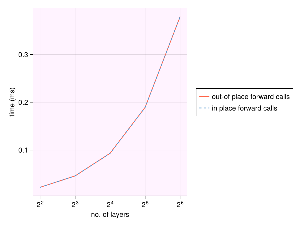

Reproducibility

The above benchmarks were obtained on AMD EPYC 9V74 80-Core Processor