Fixed discretization

Geophysical models generally have fixed discretization. This is mostly because the geophysical inverse problem is already very non-unique, and varying the discretization points together with the model values (e.g. resistivity and velocity) can make the posterior space even wider for model values. While Finite Element schemes have recently stepped in solving the corresponding PDEs, geophysical simulations have traditionally been done using finite differences which do not do well with really non-uniform discretization. Moreover, sensitivity kernels can change drastically if the cell sizes (thickness of the layers) are allowed to vary. We provide the capability to do MCMC inference on such fixed grids.

Let's denote the model parameters, eg., conductivity, by m, and the layer thickness by h. Therefore, in a N-layer case, we will have

m = [m_{1}, m_{2}, m_{3}, . . ., m_{N}] h = [h_{1}, h_{2}, h_{3}, . . ., h_{N - 1}]

such that

m_{i} \in D_{m_{i}}; where D_{m_{i}} = a priori distribution for m_{i}

and $h_{i}$ is fixed.

In the following example, we demonstrate MCMC inversion for a 3-layered earth, including the half-space being imaged using DC resistivity method. The prior distribution assumes all layers have uncorrelated resistivities bounded between $10^{- 1}$ and $10^{5}$ , defined using a uniform distribution.

!!! tip Important

The most important thing to be noted here is the specification of the prior distribution, done via:

```julia
modelD = MTModelDistribution(
    Product(
        [Uniform(-1.0, 5.0) for i in eachindex(z)]
    ),
    vec(h)
);
```

in the example.

Demo

Let's create a synthetic dataset first, with 10% error floors:

julia

m_test = DCModel(log10.([100.0, 10.0, 1000.0]), [1e3, 1e3])
locs = get_wenner_array(200:200:5000)

r_obs = forward(m_test, locs)

err_appres = 0.1 * r_obs.ρₐ
err_resp = DCResponse(err_appres)

Now, let's define the a priori with fixed grid points

julia

z = collect(0:500:2.5e3)
h = diff(z)

modelD = DCModelDistribution(Product([Uniform(-1.0, 5.0) for i in eachindex(z)]), vec(h))

then the likelihood

julia

respD = DCResponseDistribution(normal_dist)

Put everything together for MCMC

julia

n_samples = 1000
mcache = mcmc_cache(modelD, respD, n_samples, NUTS())

dc_chain = stochastic_inverse(r_obs, err_resp, locs, mcache; progress=false)

Chains MCMC chain (1000×18×1 Array{Float64, 3}):

Iterations        = 501:1:1500
Number of chains  = 1
Samples per chain = 1000
Wall duration     = 16.56 seconds
Compute duration  = 16.56 seconds
parameters        = m0[:m][1], m0[:m][2], m0[:m][3], m0[:m][4], m0[:m][5], m0[:m][6]
internals         = lp, n_steps, is_accept, acceptance_rate, log_density, hamiltonian_energy, hamiltonian_energy_error, max_hamiltonian_energy_error, tree_depth, numerical_error, step_size, nom_step_size

Summary Statistics
  parameters      mean       std      mcse   ess_bulk   ess_tail      rhat   e ⋯
      Symbol   Float64   Float64   Float64    Float64    Float64   Float64     ⋯

   m0[:m][1]    1.9970    0.0218    0.0015   178.4858   258.6622    1.0391     ⋯
   m0[:m][2]    1.9882    0.0408    0.0121    12.5368    52.7488    1.0120     ⋯
   m0[:m][3]    0.7441    0.0531    0.0214     6.2296    29.8086    1.1328     ⋯
   m0[:m][4]    3.1832    1.0099    0.2785    14.3824    21.5972    1.0863     ⋯
   m0[:m][5]    2.5697    1.4952    0.2365    51.5865   146.4764    1.0372     ⋯
   m0[:m][6]    1.5749    1.3844    0.2860    30.7530    29.2579    1.0551     ⋯
                                                                1 column omitted

Quantiles
  parameters      2.5%     25.0%     50.0%     75.0%     97.5% 
      Symbol   Float64   Float64   Float64   Float64   Float64 

   m0[:m][1]    1.9457    1.9870    1.9982    2.0078    2.0382
   m0[:m][2]    1.9302    1.9527    1.9834    2.0211    2.0638
   m0[:m][3]    0.6574    0.6955    0.7376    0.7976    0.8324
   m0[:m][4]    1.6464    2.2386    3.1681    4.0263    4.8925
   m0[:m][5]   -0.6107    1.7427    3.1874    3.6235    4.7081
   m0[:m][6]   -0.7837    0.6276    1.3624    2.4658    4.5785

The obtained dc_chain contains the a posteriori distributions that can be saved using JLD2.jl.

julia

using JLD2
JLD2.@save "file_path.jld2" dc_chain

Code for this figure

julia

fig = Figure()
ax = Axis(fig[1, 1])
hm = get_kde_image!(ax, dc_chain, modelD; kde_transformation_fn=log10,
    colormap=:binary, colorrange=(-3.0, 0.0), trans_utils=(m=no_tf, h=no_tf))
Colorbar(fig[1, 2], hm; label="log pdf")

mean_kws = (; color=:seagreen3, linewidth=2)
std_kws = (; color=:red, linewidth=1.5)
# get_mean_std_image!(ax, dc_chain, modelD; confidence_interval=0.99, trans_utils=(m=no_tf, h=no_tf), mean_kwargs=mean_kws, std_plus_kwargs=std_kws, std_minus_kwargs=std_kws)

ylims!(ax, [2500, 0])

plot_model!(ax, m_test; color=:black, linestyle=:dash, label="true", linewidth=2)
Legend(fig[2, :], ax; orientation=:horizontal)

Makie.Legend()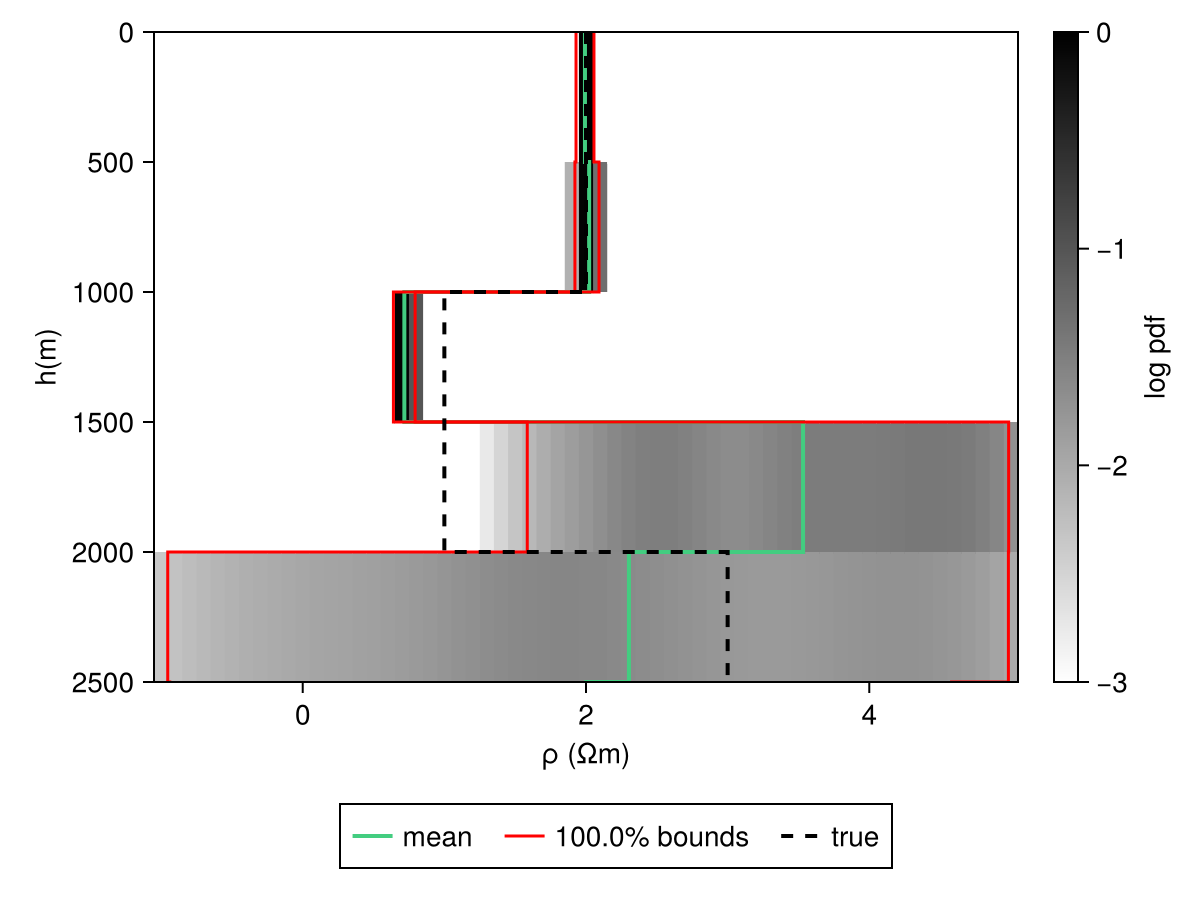

The list of models can then be obtained from chains using, which can then be used to check the fits and perform other diagnostics:

julia

model_list = get_model_list(dc_chain, modelD)

Code for this figure

julia

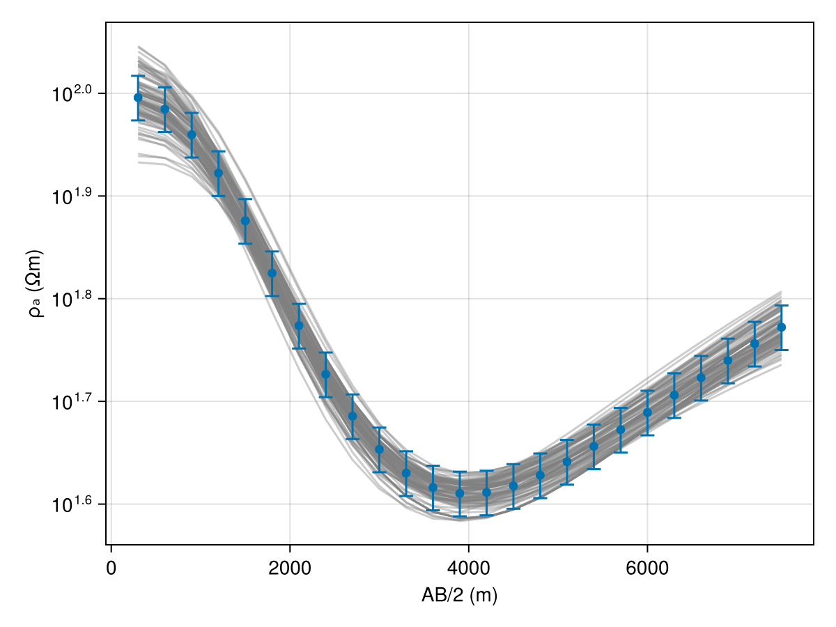
fig = Figure()
ax1 = Axis(fig[1, 1])

ab_2 = abs.(locs.srcs[:, 2] .- locs.srcs[:, 1]) ./ 2

resp_post = forward(model_list[1], locs);
for i in 1:(length(model_list) > 100 ? 100 : length(model_list))
    forward!(resp_post, model_list[i], locs)
    plot_response!([ax1], ab_2, resp_post; alpha=0.4, color=:gray)
end

plot_response!([ax1], ab_2, r_obs; errs=err_resp, plt_type=:errors, whiskerwidth=10)
plot_response!([ax1], ab_2, r_obs; plt_type=:scatter, label="true")

Fixed discretization ​

Demo ​

Fixed discretization

Demo