Occam1D

Brief introduction

We provide inversion algorithm popularized as Occam1D.

Occam1D tries to find the model with smoothest variations that fits the data. It does so by trying to minimize the first derivative of the model vector along with the misfit function. Unsurprisingly, this is done by modifying the regularizer term as

$$\begin{array}{rl}& m^T{C}_{m}m\\ =& m^T(L^{T}L)m\\ =& (Lm{)}^T(Lm)\\ =& ||Lm|{|}_2^2\end{array}$$

Occam1D also iterates over $\mu$ at every step to find the largest $\mu$ that best fits the data, steering it towards smooth models. Therefore, in every iteration, it solves for a linearized solution as well as the regularization coefficient.

Demo

We demo using Occam on a couple of models below:

Magnetotellurics (MT)

Occam1D was initially designed and compiled for 1D MT, and this is the first example we run here.

Let's define a synthetic model:

ρ = log10.([100.0, 10.0, 400.0, 1000.0])
h = [100.0, 1000.0, 10000.0]
m = MTModel(ρ, h)

1D MT Model
┌───────┬───────┬──────────┬──────────┐
│ Layer │ log-ρ │        h │        z │
│       │  [Ωm] │      [m] │      [m] │
├───────┼───────┼──────────┼──────────┤
│     1 │  2.00 │   100.00 │   100.00 │
│     2 │  1.00 │  1000.00 │  1100.00 │
│     3 │  2.60 │ 10000.00 │ 11100.00 │
│     4 │  3.00 │        ∞ │        ∞ │
└───────┴───────┴──────────┴──────────┘

and then get data, and assume 5% error floors:

T = 10 .^ (range(-1, 5; length=19))
ω = 2π ./ T
resp = forward(m, ω)

err_resp = MTResponse(0.1 .* resp.ρₐ, 180 / π .* asin(0.1) .+ zero(ω))

MTResponse{Vector{Float64}, Vector{Float64}}([1.3875320046244939, 1.0850483309402976, 1.0122693258969069, 1.3196075220402887, 2.1288222765105043, 3.742606524153418, 6.672376048265344, 11.565463875338217, 18.969398177501372, 28.926252238807752, 40.67761152951152, 52.85779579512388, 64.10592476083384, 73.57441655864378, 81.0176955269695, 86.59638574119714, 90.64544990893303, 93.52247812294203, 95.53828164509213], [5.739170477266787, 5.739170477266787, 5.739170477266787, 5.739170477266787, 5.739170477266787, 5.739170477266787, 5.739170477266787, 5.739170477266787, 5.739170477266787, 5.739170477266787, 5.739170477266787, 5.739170477266787, 5.739170477266787, 5.739170477266787, 5.739170477266787, 5.739170477266787, 5.739170477266787, 5.739170477266787, 5.739170477266787])

We need to define a data covariance matrix $C_d$ and an initial model. Let's assume gaussian noise in this case, and choose an initial model a half-space of 100 $\mathrm{\Omega }m$.

C_d = diagm(inv.([err_resp.ρₐ..., err_resp.ϕ...])) .^ 2; # weight matrix

# initial model
h_test = 10 .^ range(0.0, 5.0; length=50)
ρ_test = 2 .* ones(length(h_test) + 1)

m_occam = MTModel(ρ_test, h_test);

1D MT Model
┌───────┬───────┬────────┬────────┐
│ Layer │ log-ρ │      h │      z │
│       │  [Ωm] │    [m] │    [m] │
├───────┼───────┼────────┼────────┤
│     1 │  2.00 │   1.00 │   1.00 │
│     2 │  2.00 │   1.26 │   2.27 │
│     3 │  2.00 │   1.60 │   3.87 │
│     4 │  2.00 │   2.02 │   5.89 │
│     5 │  2.00 │   2.56 │   8.45 │
│     6 │  2.00 │   3.24 │  11.69 │
│     7 │  2.00 │   4.09 │  15.78 │
│     8 │  2.00 │   5.18 │  20.96 │
│     9 │  2.00 │   6.55 │  27.51 │
│    10 │  2.00 │   8.29 │  35.80 │
│    11 │  2.00 │  10.48 │  46.28 │
│    12 │  2.00 │  13.26 │  59.54 │
│    13 │  2.00 │  16.77 │  76.30 │
│    14 │  2.00 │  21.21 │  97.51 │
│   ⋮   │   ⋮   │   ⋮    │   ⋮    │
└───────┴───────┴────────┴────────┘
                    37 rows omitted

The final result will be stored in the same variable m_occam. All we need to do now is specify using Occam and then calling inverse!.

Note

Using Occam, you also have the option to perform a smoothing step. Once the model has achieved the threshold misfit, it is smoothened until it fits the data just about the threshold misfit.

alg_cache = Occam(; μgrid=[1e-2, 1e6])
inverse!(
    m_occam, resp, ω, alg_cache; W=C_d, max_iters=50, verbose=true, smoothing_step=true)

PrISM.return_code{MTModel{Vector{Float64}, Vector{Float64}}}(true, (μ = 16.68184405948691,), 1D MT Model
┌───────┬───────┬────────┬────────┐
│ Layer │ log-ρ │      h │      z │
│       │  [Ωm] │    [m] │    [m] │
├───────┼───────┼────────┼────────┤
│     1 │  1.07 │   1.00 │   1.00 │
│     2 │  1.07 │   1.26 │   2.27 │
│     3 │  1.07 │   1.60 │   3.87 │
│     4 │  1.07 │   2.02 │   5.89 │
│     5 │  1.07 │   2.56 │   8.45 │
│     6 │  1.07 │   3.24 │  11.69 │
│     7 │  1.07 │   4.09 │  15.78 │
│     8 │  1.07 │   5.18 │  20.96 │
│     9 │  1.07 │   6.55 │  27.51 │
│    10 │  1.07 │   8.29 │  35.80 │
│    11 │  1.07 │  10.48 │  46.28 │
│    12 │  1.06 │  13.26 │  59.54 │
│    13 │  1.06 │  16.77 │  76.30 │
│    14 │  1.06 │  21.21 │  97.51 │
│   ⋮   │   ⋮   │   ⋮    │   ⋮    │
└───────┴───────┴────────┴────────┘
                    37 rows omitted
, 1.0, 0.9879974070792524)

Code for this figure

fig = Figure()
ax_m = Axis(fig[1:2, 1]; yscale=log10)

plot_model!(ax_m, m; label="true", color=:steelblue3)
plot_model!(ax_m, m_occam; label="occam", color=:tomato)
fig

ax1 = Axis(fig[1, 2]; xscale=log10)
ax2 = Axis(fig[2, 2]; xscale=log10)

plot_response!([ax1, ax2], T, resp; plt_type=:scatter, color=:steelblue3)
plot_response!([ax1, ax2], T, resp; errs=err_resp, plt_type=:errors,
    whiskerwidth=10, color=:steelblue3)

resp_occam = forward(m_occam, ω)
plot_response!([ax1, ax2], T, resp_occam; color=:tomato)
Legend(fig[3, :], ax_m; orientation=:horizontal)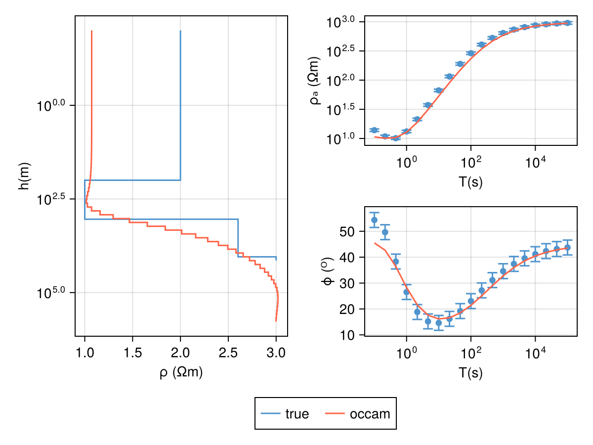

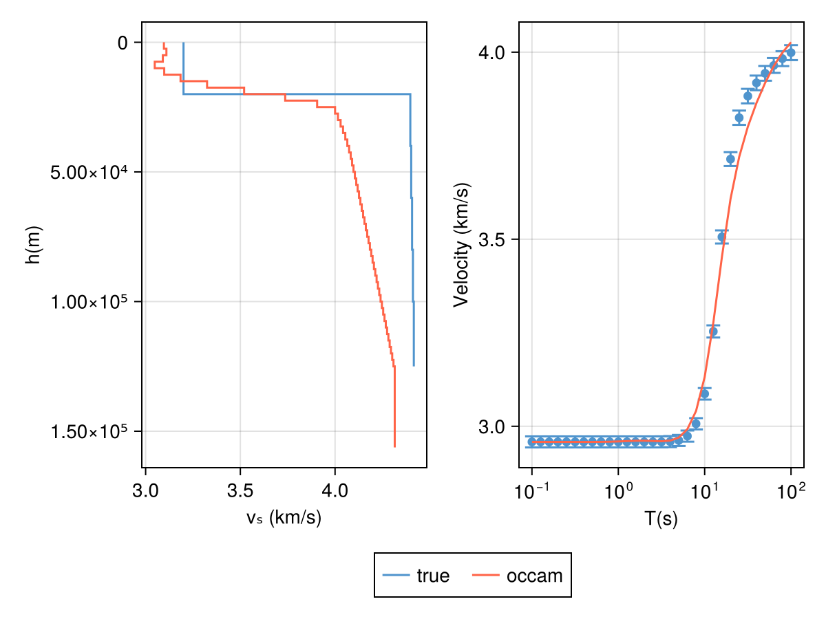
Rayleigh waves

Let's also do an Occam inversion on Rayleigh waves. Like before, we define a synthetic model :

vs = [3.2, 4.39731, 4.40192, 4.40653, 4.41113, 4.41574]
vp = [5.8, 8.01571, 7.99305, 7.97039, 7.94773, 7.92508]
ρ = [2.6, 3.38014, 3.37797, 3.37579, 3.37362, 3.37145]
h = [20.0, 20.0, 20.0, 20.0, 20.0] .* 1e3
m = RWModel(vs, h, ρ, vp)

1D Rayleigh Wave Model
┌───────┬────────┬──────────┬───────────┬──────────┬────────┐
│ Layer │     vₛ │        h │         z │        ρ │     vₚ │
│       │ [km/s] │      [m] │       [m] │ [kg⋅m⁻³] │ [km/s] │
├───────┼────────┼──────────┼───────────┼──────────┼────────┤
│     1 │   3.20 │ 20000.00 │  20000.00 │      2.6 │    5.8 │
│     2 │   4.40 │ 20000.00 │  40000.00 │     3.38 │  8.016 │
│     3 │   4.40 │ 20000.00 │  60000.00 │    3.378 │  7.993 │
│     4 │   4.41 │ 20000.00 │  80000.00 │    3.376 │   7.97 │
│     5 │   4.41 │ 20000.00 │ 100000.00 │    3.374 │  7.948 │
│     6 │   4.42 │        ∞ │         ∞ │    3.371 │  7.925 │
└───────┴────────┴──────────┴───────────┴──────────┴────────┘

and then get the forward response, with 1% error floors :

freq = exp10.(-2:0.1:1)
t = inv.(freq)

resp = forward(m, t)

err_resp = SurfaceWaveResponse(0.01 .* resp.c,)

SurfaceWaveResponse{Vector{Float64}}([0.03998742809891679, 0.039827418196201114, 0.03964482211470584, 0.039434630930423535, 0.039178924423455996, 0.03882648753523808, 0.038248044675588434, 0.03714191050529465, 0.03506108998060216, 0.032535215306282  …  0.03207548274397846, 0.03204606792330738, 0.03202832164168354, 0.03215848099589343, 0.03209821282029148, 0.032061115247011135, 0.032347990459203675, 0.032456859511136964, 0.03201496360898014, 0.03208482858538624])

Then we declare an initial model, and define the error covariance matrix :

h_test = fill(2500.0, 50)
m_occam = RWModel(4.0 .+ zeros(length(h_test) + 1), h_test, fill(3e3, 51), fill(7e3, 51))

C_d = diagm(inv.(err_resp.c)) .^ 2

and perform the inversion:

alg_cache = Occam(; μgrid=[1e-2, 1e2])
rw_bounds = transform_utils(
    x -> SubsurfaceCore.sigmoid(x, 3.0, 5.0), x -> SubsurfaceCore.inverse_sigmoid(x, 3.0, 5.0))
retcode = inverse!(m_occam, resp, t, alg_cache; W=C_d, max_iters=100,
    verbose=true, model_trans_utils=rw_bounds);

PrISM.return_code{RWModel{Vector{Float64}, Vector{Float64}, Vector{Float64}, Vector{Float64}}}(false, (μ = 0.047089272184461274,), 1D Rayleigh Wave Model
┌───────┬────────┬─────────┬──────────┬──────────┬────────┐
│ Layer │     vₛ │       h │        z │        ρ │     vₚ │
│       │ [km/s] │     [m] │      [m] │ [kg⋅m⁻³] │ [km/s] │
├───────┼────────┼─────────┼──────────┼──────────┼────────┤
│     1 │   3.36 │ 2500.00 │  2500.00 │   3000.0 │ 7000.0 │
│     2 │   3.46 │ 2500.00 │  5000.00 │   3000.0 │ 7000.0 │
│     3 │   4.18 │ 2500.00 │  7500.00 │   3000.0 │ 7000.0 │
│     4 │   4.11 │ 2500.00 │ 10000.00 │   3000.0 │ 7000.0 │
│     5 │   3.40 │ 2500.00 │ 12500.00 │   3000.0 │ 7000.0 │
│     6 │   3.04 │ 2500.00 │ 15000.00 │   3000.0 │ 7000.0 │
│     7 │   3.00 │ 2500.00 │ 17500.00 │   3000.0 │ 7000.0 │
│     8 │   4.68 │ 2500.00 │ 20000.00 │   3000.0 │ 7000.0 │
│     9 │   4.98 │ 2500.00 │ 22500.00 │   3000.0 │ 7000.0 │
│    10 │   3.00 │ 2500.00 │ 25000.00 │   3000.0 │ 7000.0 │
│    11 │   3.04 │ 2500.00 │ 27500.00 │   3000.0 │ 7000.0 │
│    12 │   4.09 │ 2500.00 │ 30000.00 │   3000.0 │ 7000.0 │
│    13 │   4.10 │ 2500.00 │ 32500.00 │   3000.0 │ 7000.0 │
│    14 │   4.11 │ 2500.00 │ 35000.00 │   3000.0 │ 7000.0 │
│   ⋮   │   ⋮    │    ⋮    │    ⋮     │    ⋮     │   ⋮    │
└───────┴────────┴─────────┴──────────┴──────────┴────────┘
                                            37 rows omitted
, 1.0, 5.367608586079127)

Code for this figure

fig = Figure()
ax_m = Axis(fig[1, 1]; xlabel="Vs (km/s)", ylabel="depth (m)")

plot_model!(ax_m, m; label="true", color=:steelblue3)
plot_model!(ax_m, m_occam; label="occam", color=:tomato)
fig

ax1 = Axis(fig[1, 2]; xscale=log10)

plot_response!([ax1], t, resp; plt_type=:scatter, color=:steelblue3)
plot_response!(
    [ax1], t, resp; errs=err_resp, plt_type=:errors, whiskerwidth=10, color=:steelblue3)

resp_occam = forward(m_occam, t)
plot_response!([ax1], t, resp_occam; color=:tomato)
Legend(fig[2, :], ax_m; orientation=:horizontal)